Chapter 11 Visualization
XMAS 2.0 provides mulitple functions for visualization. For instance, using plot_volcano to display the results of differential analysis.
Outline of this Chapter:
11.2 Importing Data
data("amplicon_ps")
amplicon_ps_rarefy <- norm_rarefy(object = amplicon_ps,
                                  size = 1114)
amplicon_ps_rarefy
## phyloseq-class experiment-level object
## otu_table() OTU Table: [ 2308 taxa and 34 samples ]
## sample_data() Sample Data: [ 34 samples by 8 sample variables ]
## tax_table() Taxonomy Table: [ 2308 taxa by 7 taxonomic ranks ]
## phy_tree() Phylogenetic Tree: [ 2308 tips and 2306 internal nodes ]11.3 plot_boxplot
- calculate alpha diversity
dat_alpha <- run_alpha_diversity(ps = amplicon_ps_rarefy,
                                 measures = c("Shannon", "Chao1", "Observed"))
head(dat_alpha)
## TempRowNames SampleType Year Month Day Subject ReportedAntibioticUsage DaysSinceExperimentStart Description Observed Chao1
## 1 L1S140 gut 2008 10 28 2 Yes 0 2_Fece_10_28_2008 27 74.50
## 2 L1S208 gut 2009 1 20 2 No 84 2_Fece_1_20_2009 40 148.75
## 3 L1S8 gut 2008 10 28 1 Yes 0 1_Fece_10_28_2008 19 54.00
## 4 L1S281 gut 2009 4 14 2 No 168 2_Fece_4_14_2009 60 256.00
## 5 L3S242 right palm 2008 10 28 1 Yes 0 1_R_Palm_10_28_2008 16 42.00
## 6 L2S309 left palm 2009 1 20 2 No 84 2_L_Palm_1_20_2009 12 57.00
## se.chao1 Shannon
## 1 30.70970 3.126005
## 2 62.86107 3.303186
## 3 25.57190 2.688337
## 4 93.42352 3.664947
## 5 19.97805 2.692311
## 6 30.06061 2.082828plot_boxplot has many parameters, and help you enjoy it.
- single measure

Figure 11.1: boxplot(single measure)
- single measure with significant results
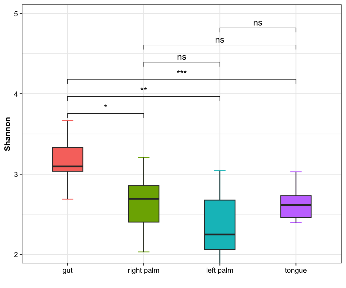
Figure 11.2: boxplot(single measure with significant results)
- single measure with significant results of pairwises
plot_boxplot(data = dat_alpha,
             y_index = "Shannon",
             group = "SampleType",
             do_test = TRUE,
             cmp_list = list(c("gut", "right palm"),
                             c("gut", "tongue")))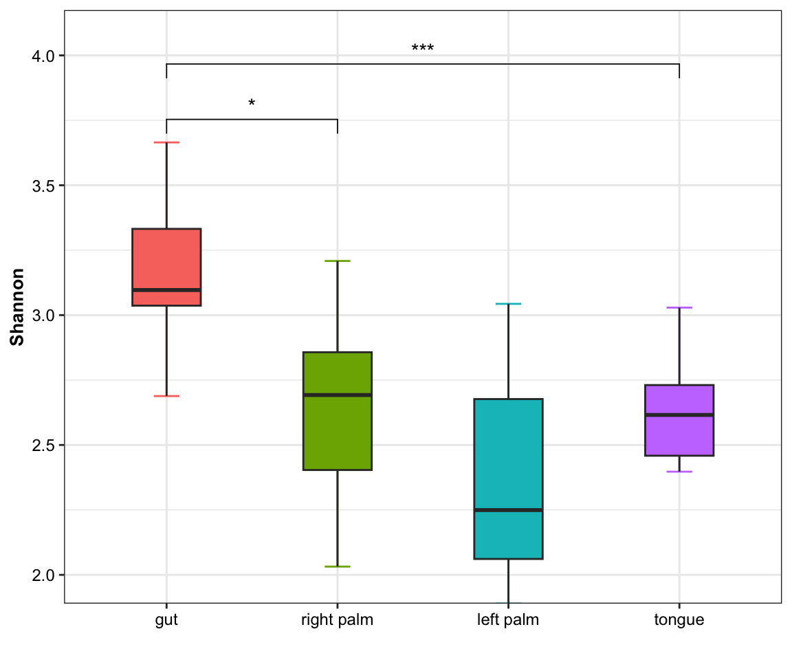
Figure 11.3: boxplot(single measure with significant results of pairwises)
- single measure with significant results of pairwises and outlier
plot_boxplot(data = dat_alpha,
             y_index = "Shannon",
             group = "SampleType",
             do_test = TRUE,
             cmp_list = list(c("gut", "right palm"),
                             c("gut", "tongue")),
             outlier = TRUE)
Figure 11.4: boxplot(single measure with significant results of pairwises and outlier)
- single measure with significant results of ref_group
plot_boxplot(data = dat_alpha,
             y_index = "Shannon",
             group = "SampleType",
             do_test = TRUE,
             ref_group = "gut")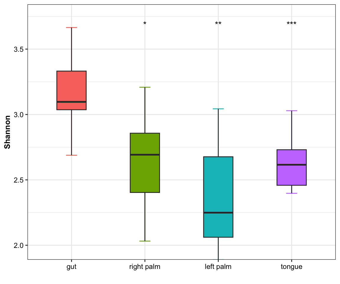
Figure 11.5: boxplot(single measure with significant results of ref_group)
- multiple measures
plot_boxplot(data = dat_alpha,
             y_index = c("Shannon", "Chao1", "Observed"),
             group = "SampleType",
             group_names = c("gut", "right palm", "tongue"),
             group_color = c("red", "green", "blue"),
             ref_group = "gut",
             method = "wilcox.test",
             outlier = TRUE)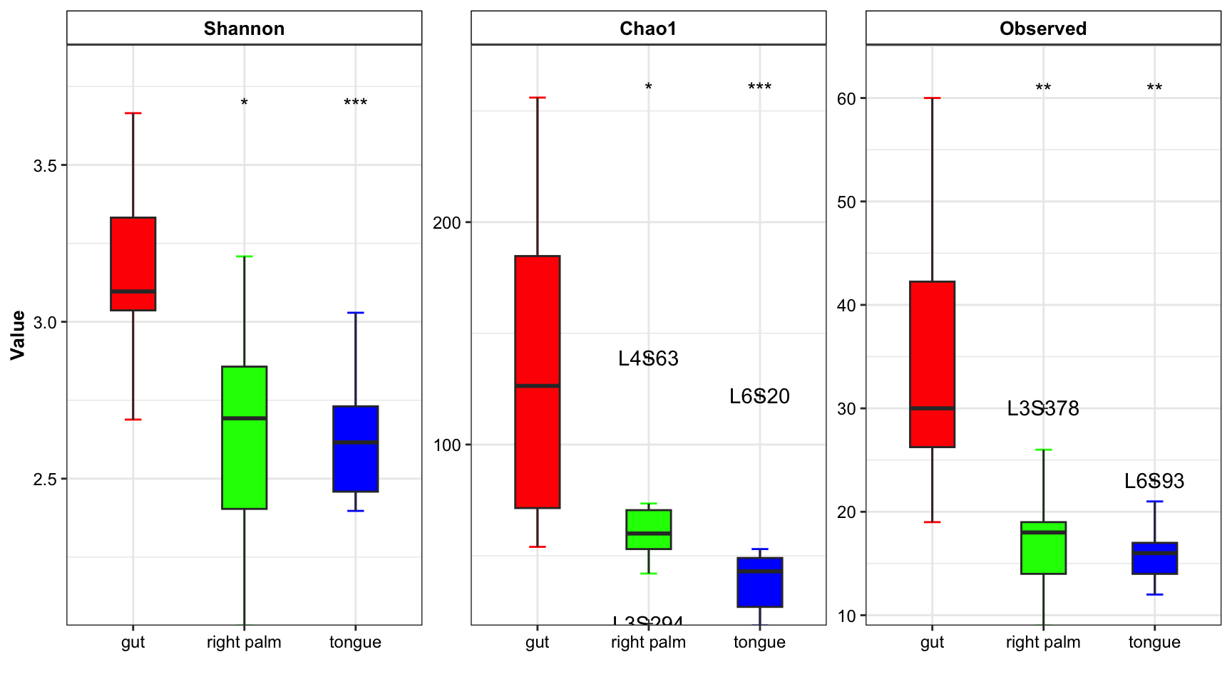
Figure 11.6: boxplot(multiple measure with group number)
- show group_number in the x-axis break
plot_boxplot(data = dat_alpha,
             y_index = c("Shannon", "Chao1", "Observed"),
             group = "SampleType",
             group_names = c("gut", "right palm", "tongue"),
             group_color = c("red", "green", "blue"),
             do_test = TRUE,
             method = "wilcox.test",
             group_number = TRUE)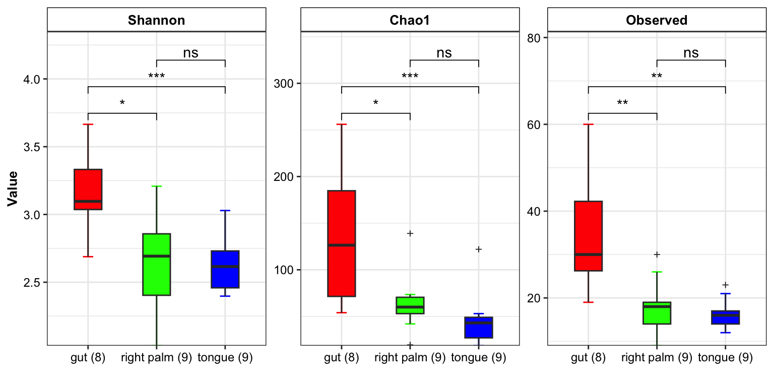
Figure 11.7: boxplot(group_number)
11.4 plot_barplot
plot_barplot has many parameters, and help you enjoy it.
- single measure
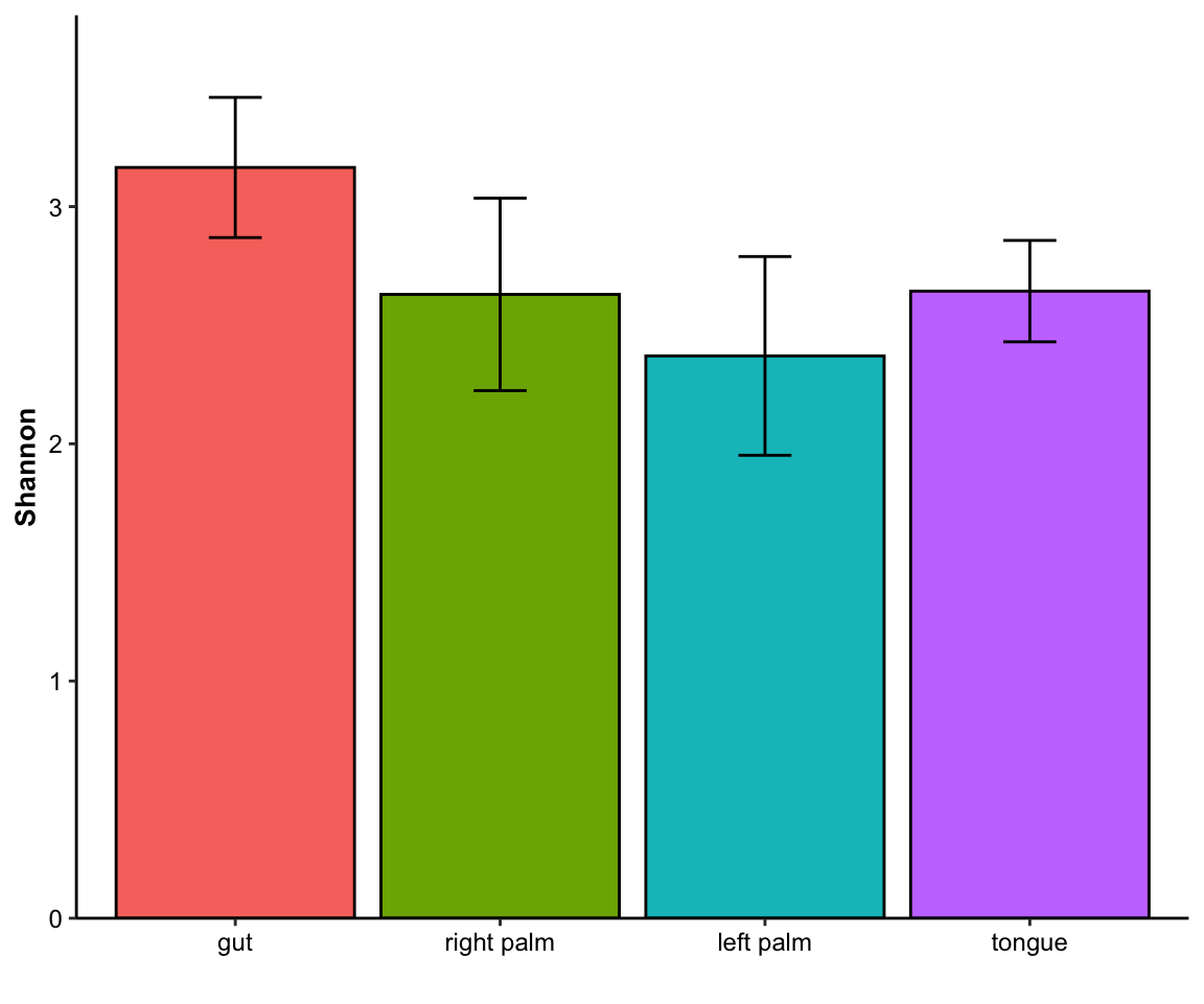
Figure 11.8: barplot(single measure)
- single measure with significant results
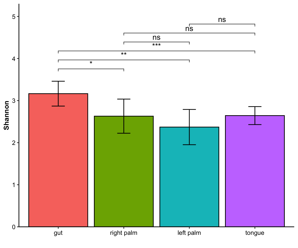
Figure 11.9: barplot(single measure with significant results)
- single measure with significant results of pairwises
plot_barplot(data = dat_alpha,
             y_index = "Shannon",
             group = "SampleType",
             do_test = TRUE,
             cmp_list = list(c("gut", "right palm"), c("gut", "tongue")))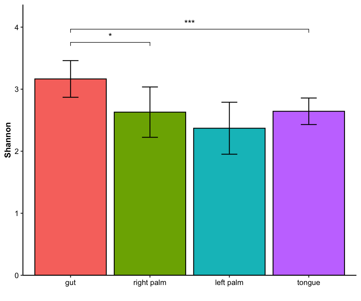
Figure 11.10: barplot(single measure with significant results of pairwises)
- single measure with significant results of ref_group
plot_barplot(data = dat_alpha,
             y_index = "Shannon",
             group = "SampleType",
             do_test = TRUE,
             ref_group = "gut")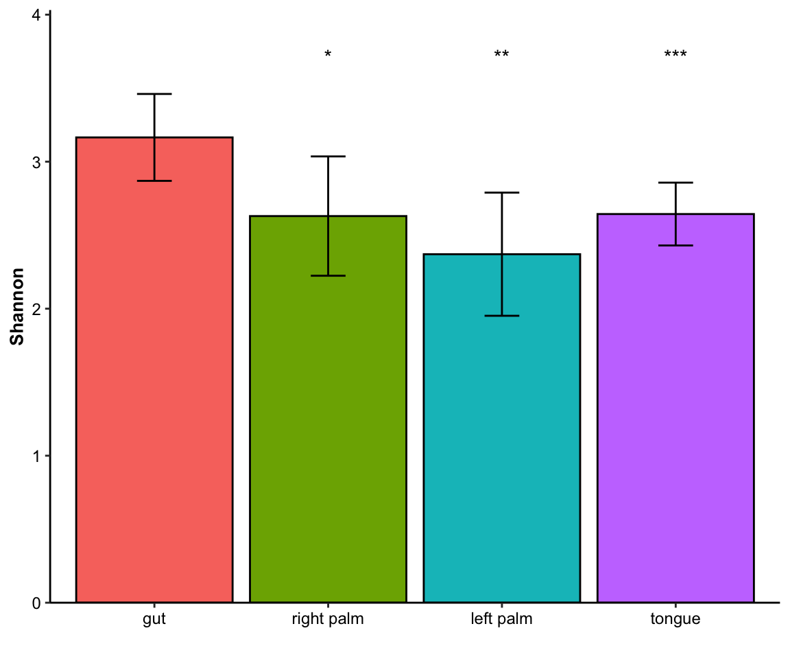
Figure 11.11: barplot(single measure with significant results of ref_group)
- multiple index
plot_barplot(data = dat_alpha,
             y_index = c("Shannon", "Chao1", "Observed"),
             group = "SampleType",
             do_test = TRUE,
             method = "wilcox.test")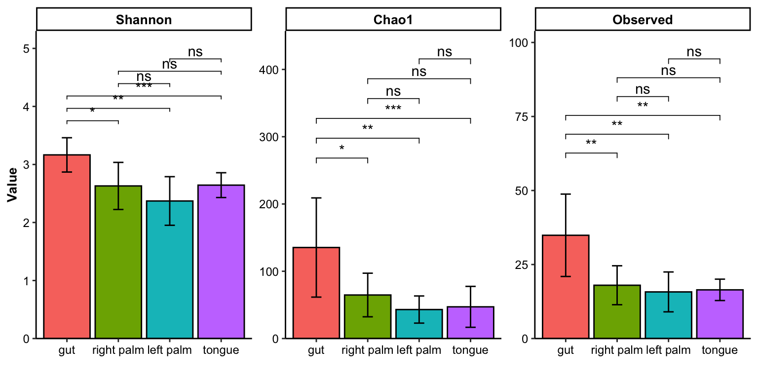
Figure 11.12: barplot(multiple index)
- show group_number in the x-axis break
plot_barplot(data = dat_alpha,
             y_index = c("Shannon", "Chao1", "Observed"),
             group = "SampleType",
             group_names = c("gut", "right palm", "tongue"),
             group_color = c("red", "green", "blue"),
             do_test = TRUE,
             method = "wilcox.test",
             group_number = TRUE)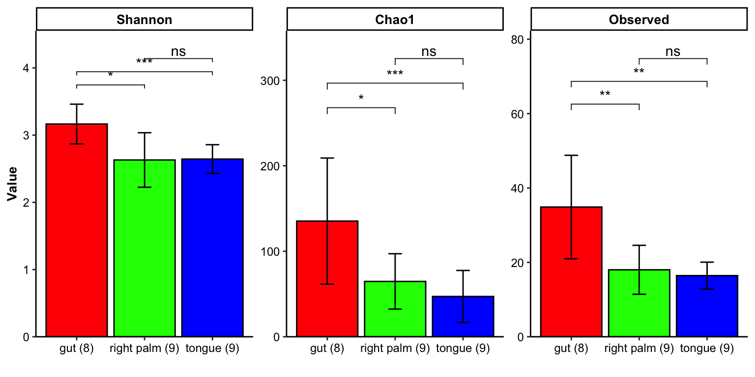
Figure 11.13: barplot(group_number)
11.5 plot_dotplot
plot_dotplot has many parameters, and help you enjoy it.
- single measure
## Bin width defaults to 1/30 of the range of the data. Pick better value with `binwidth`.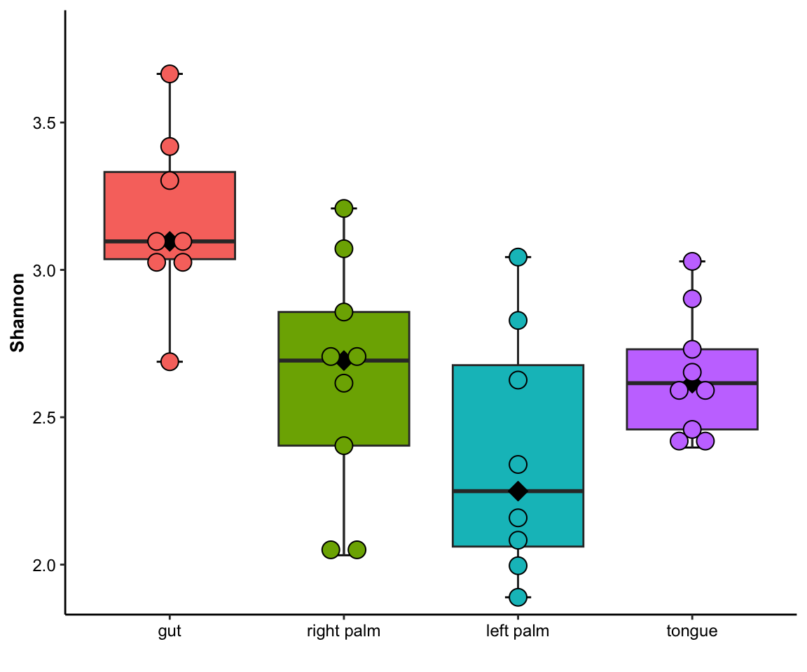
Figure 11.14: dotplot(single measure)
- single measure with significant results
## Bin width defaults to 1/30 of the range of the data. Pick better value with `binwidth`.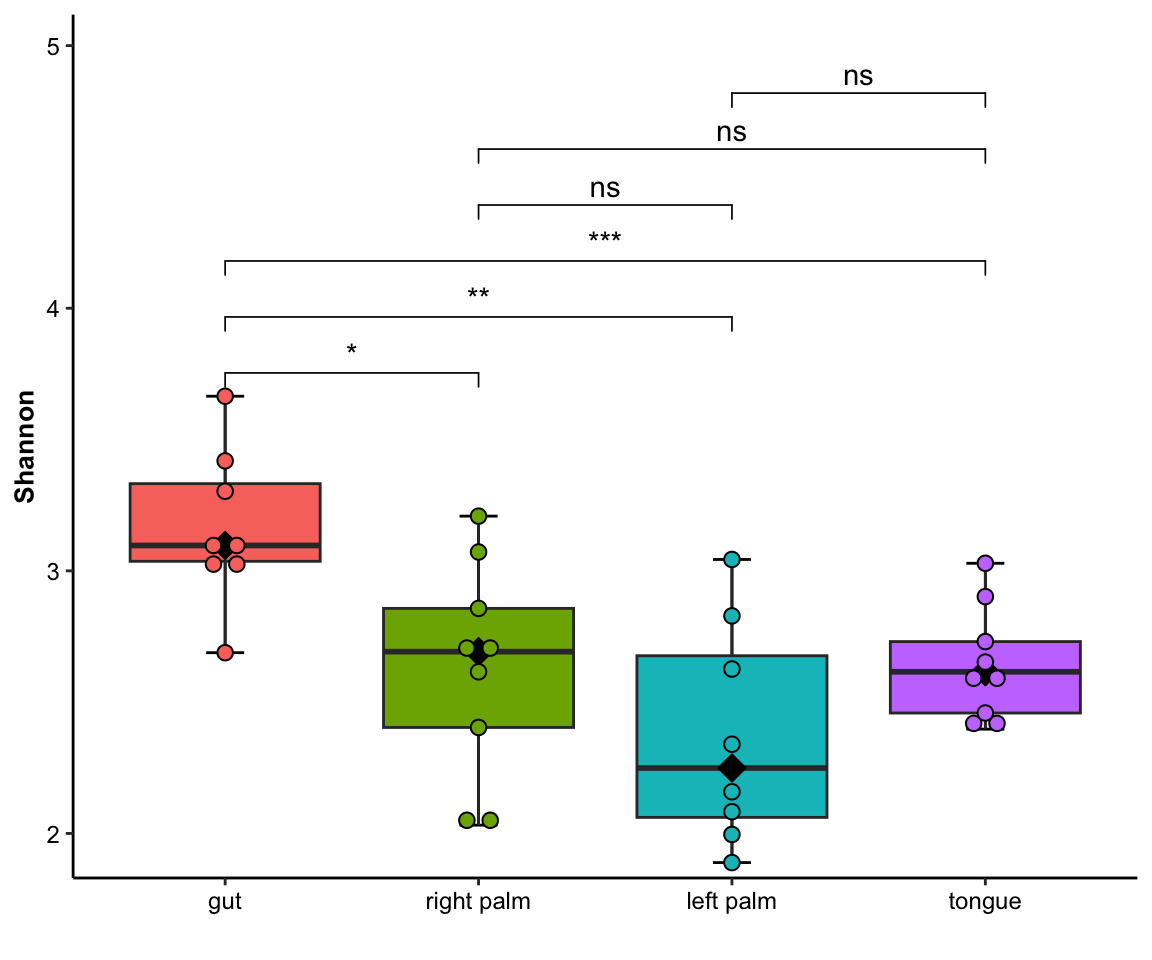
Figure 11.15: dotplot(single measure with significant results)
- single measure with significant results of pairwises
plot_dotplot(data = dat_alpha,
             y_index = "Shannon",
             group = "SampleType",
             do_test = TRUE,
             cmp_list = list(c("gut", "right palm"),
                             c("gut", "tongue")))
## Bin width defaults to 1/30 of the range of the data. Pick better value with `binwidth`.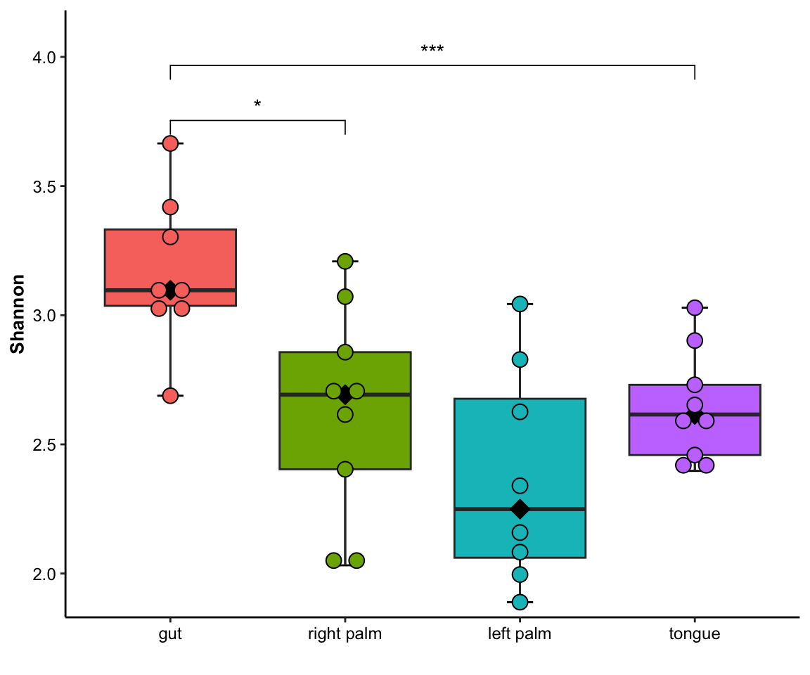
Figure 11.16: dotplot(single measure with significant results of pairwises)
- single measure with significant results of ref_group
plot_dotplot(
    data = dat_alpha,
    y_index = "Shannon",
    group = "SampleType",
    do_test = TRUE,
    ref_group = "gut")
## Bin width defaults to 1/30 of the range of the data. Pick better value with `binwidth`.
Figure 11.17: dotplot(single measure with significant results of ref_group)
- dot size and median size
plot_dotplot(
    data = dat_alpha,
    y_index = "Shannon",
    group = "SampleType",
    do_test = TRUE,
    ref_group = "gut",
    dotsize = 0.5,
    mediansize = 2)
## Bin width defaults to 1/30 of the range of the data. Pick better value with `binwidth`.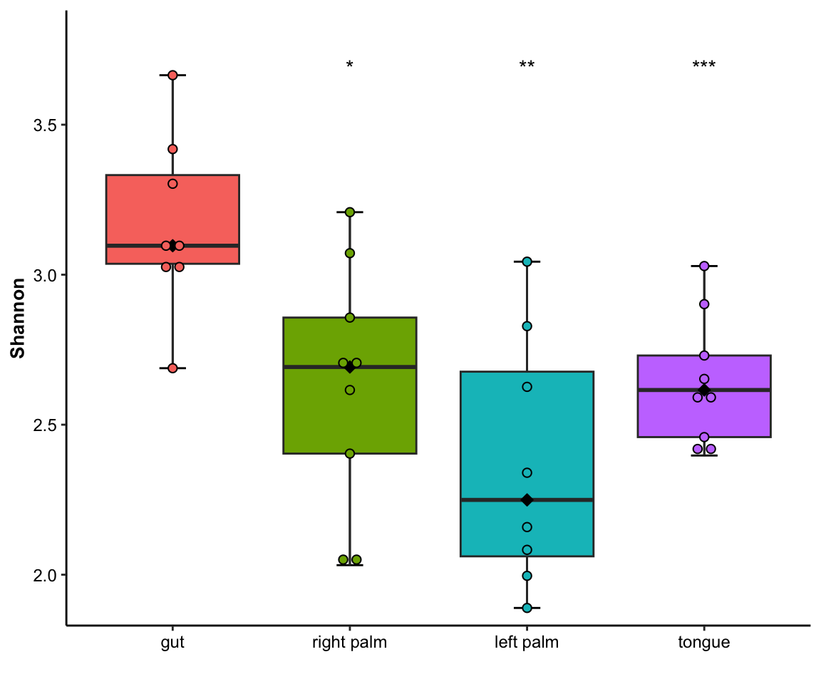
Figure 11.18: dotplot(dot size and median size)
- multiple index
plot_dotplot(
    data = dat_alpha,
    y_index = c("Shannon", "Chao1", "Observed"),
    group = "SampleType",
    do_test = TRUE,
    method = "wilcox.test")
## Bin width defaults to 1/30 of the range of the data. Pick better value with `binwidth`.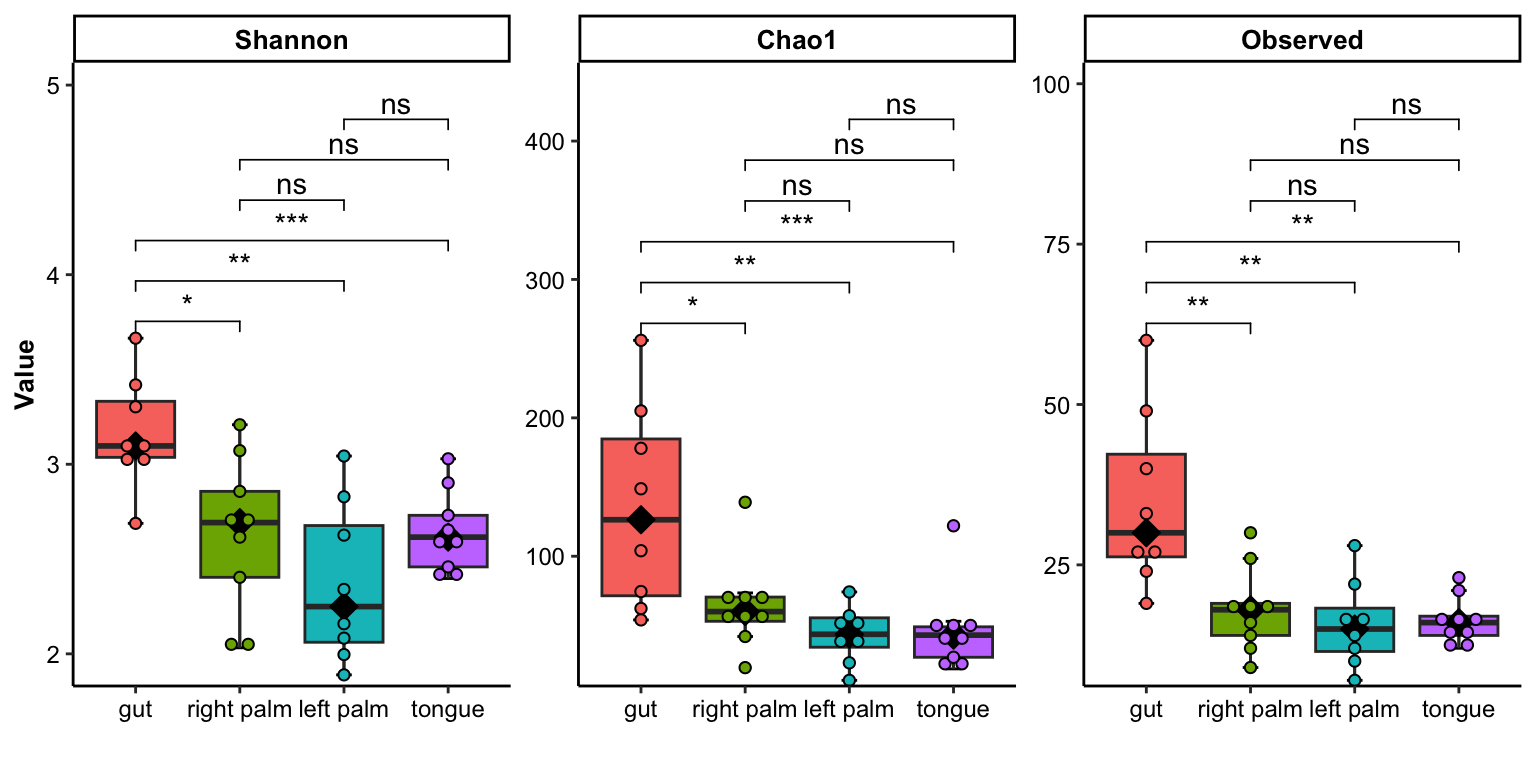
Figure 11.19: dotplot(multiple index)
- multiple index with errorbar
plot_dotplot(
    data = dat_alpha,
    y_index = c("Shannon", "Chao1", "Observed"),
    group = "SampleType",
    do_test = TRUE,
    show_type = "errorbar",
    method = "wilcox.test")
## Bin width defaults to 1/30 of the range of the data. Pick better value with `binwidth`.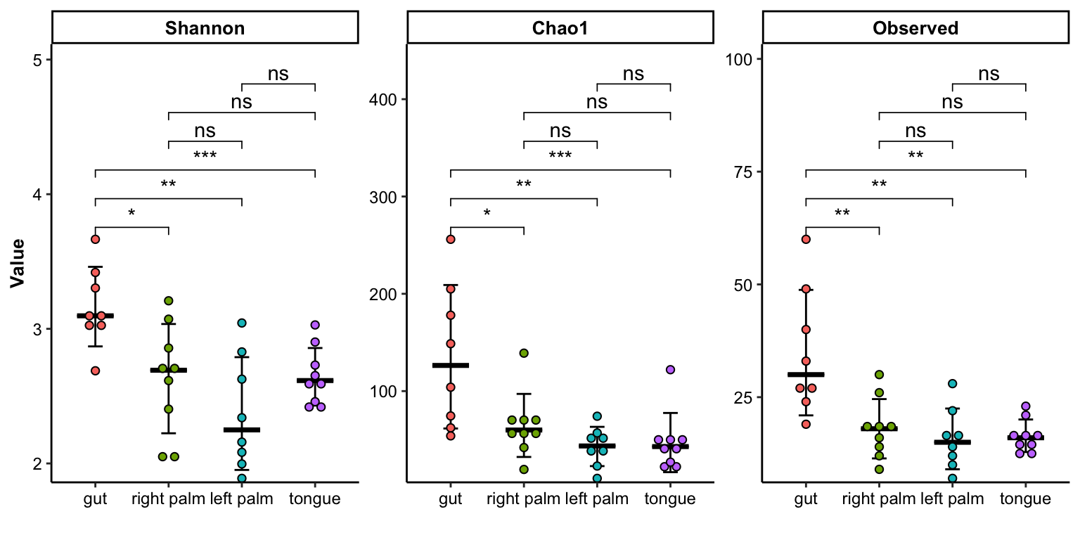
Figure 11.20: dotplot(multiple index errorbar)
- show group_number in the x-axis break
plot_dotplot(data = dat_alpha,
             y_index = c("Shannon", "Chao1", "Observed"),
             group = "SampleType",
             group_names = c("gut", "right palm", "tongue"),
             group_color = c("red", "green", "blue"),
             show_type = "errorbar",
             do_test = TRUE,
             method = "wilcox.test",
             group_number = TRUE)
## Bin width defaults to 1/30 of the range of the data. Pick better value with `binwidth`.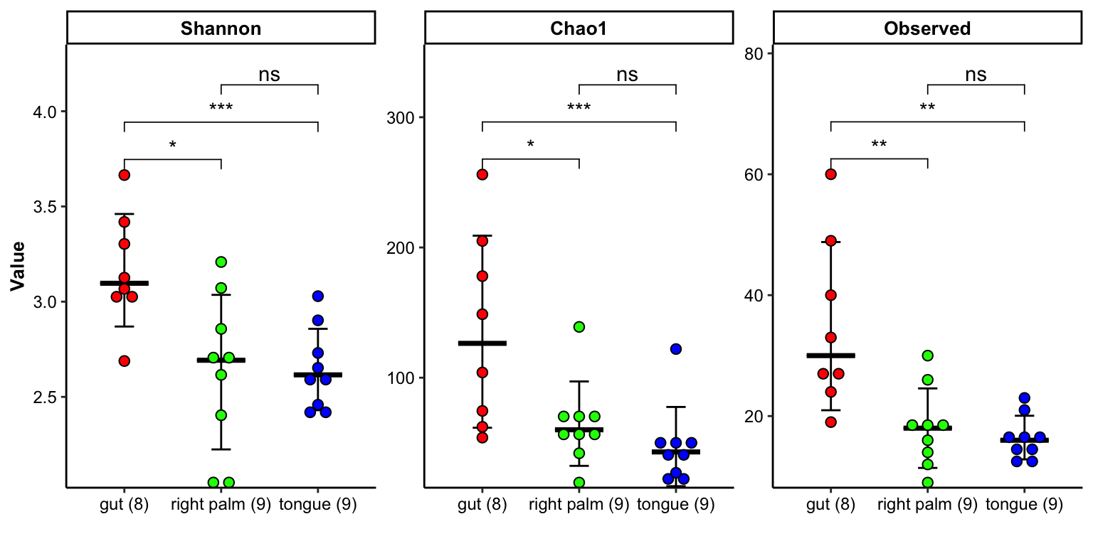
Figure 11.21: dotplot(group_number)
11.6 plot_correlation_boxplot
Help you enjoy plot_correlation_boxplot.
plot_correlation_boxplot(
    data = dat_alpha,
    x_index = "Chao1",
    y_index = "Shannon",
    group = "SampleType")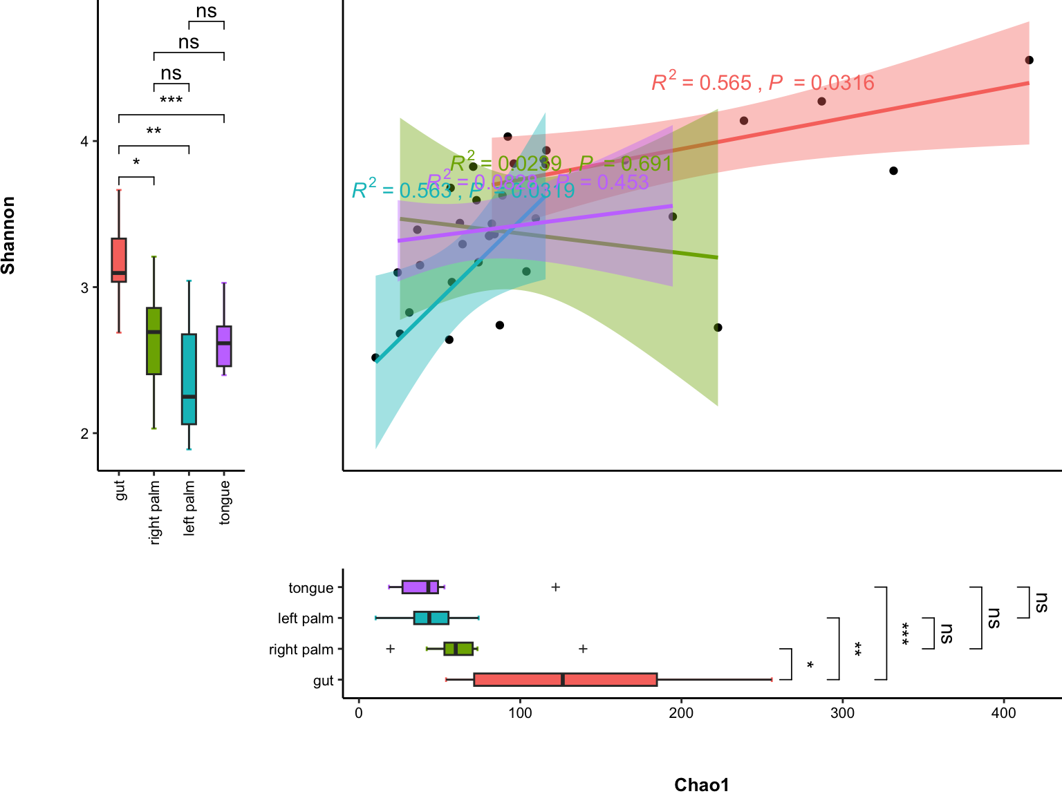
Figure 11.22: correlation with boxplot
11.7 plot_correlation_density
Help you enjoy plot_correlation_density.
plot_correlation_density(
    data = dat_alpha,
    x_index = "Chao1",
    y_index = "Shannon",
    group = "SampleType")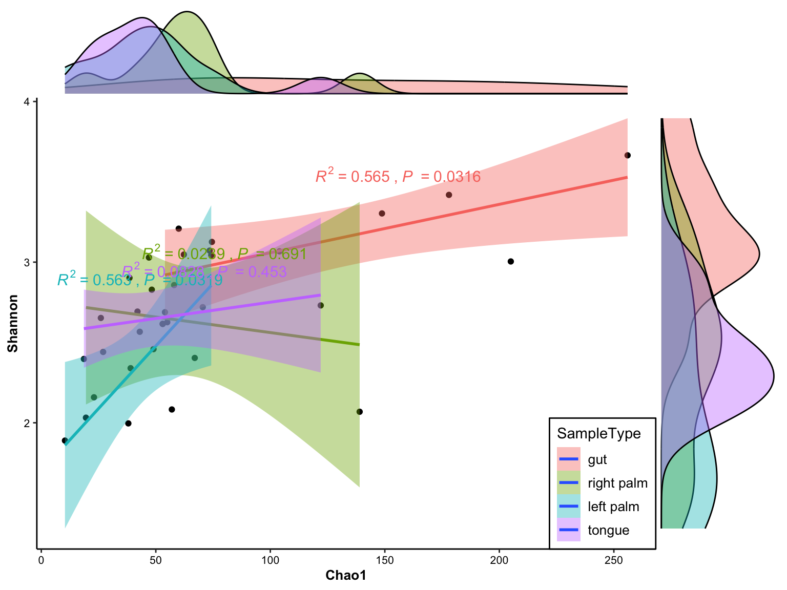
Figure 11.23: correlation with density
11.8 plot_Ordination
plot_Ordination provides too many parameters for users to display the ordination results by using ggplot2 format. Here is the ordinary pattern.
data("dada2_ps")

# step1: Removing samples of specific group in phyloseq-class object
dada2_ps_remove_BRS <- get_GroupPhyloseq(
                     ps = dada2_ps,
                     group = "Group",
                     group_names = "QC")

# step2: Rarefying counts in phyloseq-class object
dada2_ps_rarefy <- norm_rarefy(object = dada2_ps_remove_BRS,
                               size = 51181)

# step3: Extracting specific taxa phyloseq-class object
dada2_ps_rare_genus <- summarize_taxa(ps = dada2_ps_rarefy,
                                      taxa_level = "Genus",
                                      absolute = TRUE)

# step4: Aggregating low relative abundance or unclassified taxa into others
# dada2_ps_genus_LRA <- summarize_LowAbundance_taxa(ps = dada2_ps_rare_genus,
#                                                   cutoff = 10,
#                                                   unclass = TRUE)

# step4: Filtering the low relative abundance or unclassified taxa by the threshold
dada2_ps_genus_filter <- run_filter(ps = dada2_ps_rare_genus,
                                    cutoff = 10,
                                    unclass = TRUE)

# step5: Trimming the taxa with low occurrence less than threshold
dada2_ps_genus_filter_trim <- run_trim(object = dada2_ps_genus_filter,
                                       cutoff = 0.2,
                                       trim = "feature")
dada2_ps_genus_filter_trim
## phyloseq-class experiment-level object
## otu_table() OTU Table: [ 83 taxa and 23 samples ]
## sample_data() Sample Data: [ 23 samples by 1 sample variables ]
## tax_table() Taxonomy Table: [ 83 taxa by 6 taxonomic ranks ]ordination_PCA <- run_ordination(
ps = dada2_ps_genus_filter_trim,
group = "Group",
method = "PCA")
names(ordination_PCA)## [1] "fit" "dat" "explains" "eigvalue" "PERMANOVA" "BETADISPER" "axis_taxa_cor"- Ordinary pattern
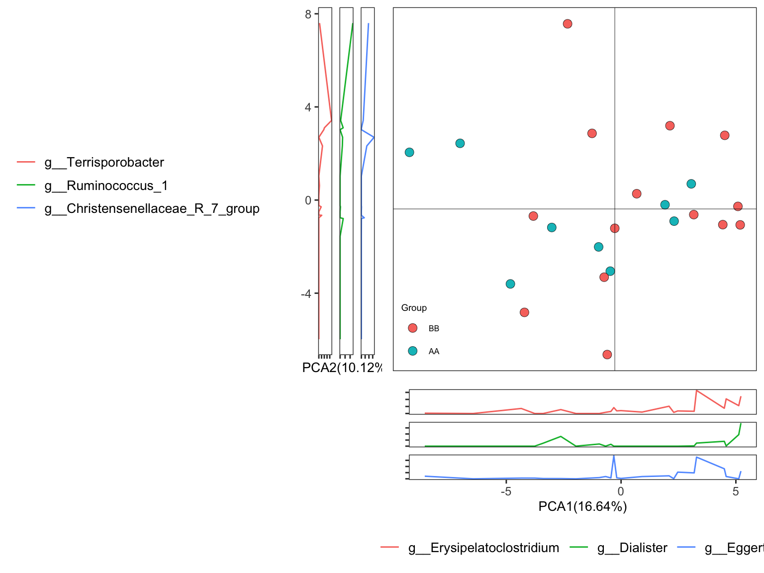
Figure 11.24: plot_Ordination (Ordinary pattern)
- plot with SampleID and setting group colors
plot_Ordination(ResultList = ordination_PCA,
                group = "Group",
                group_names = c("AA", "BB"),
                group_color = c("blue", "red"),
                circle_type = "ellipse",
                sample = TRUE)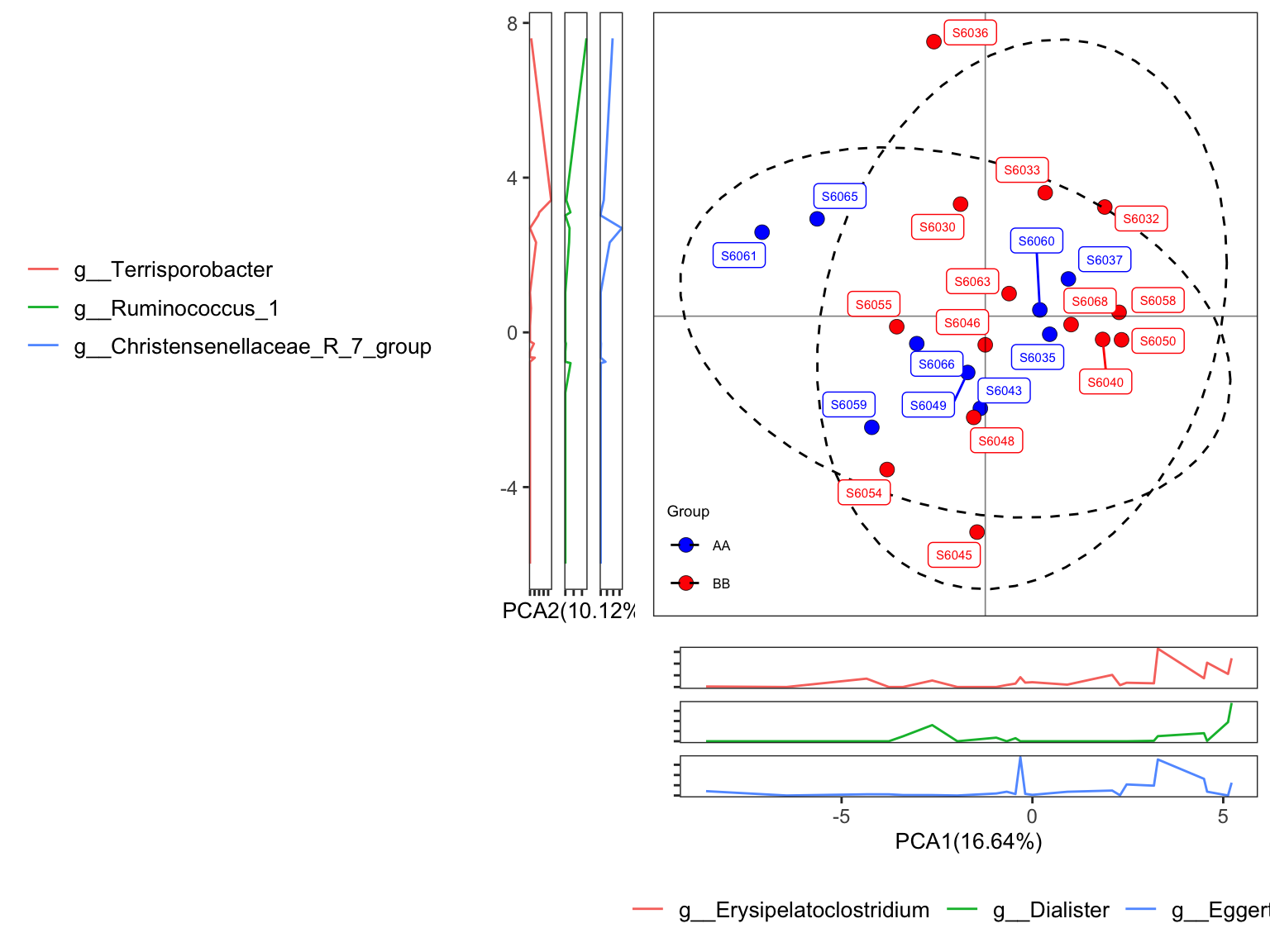
Figure 11.25: plot_Ordination (Ordinary pattern with SampleID)
- ellipse with 95% confidence interval
plot_Ordination(ResultList = ordination_PCA,
                group = "Group",
                group_names = c("AA", "BB"),
                group_color = c("blue", "red"),
                circle_type = "ellipse_CI",
                sample = TRUE)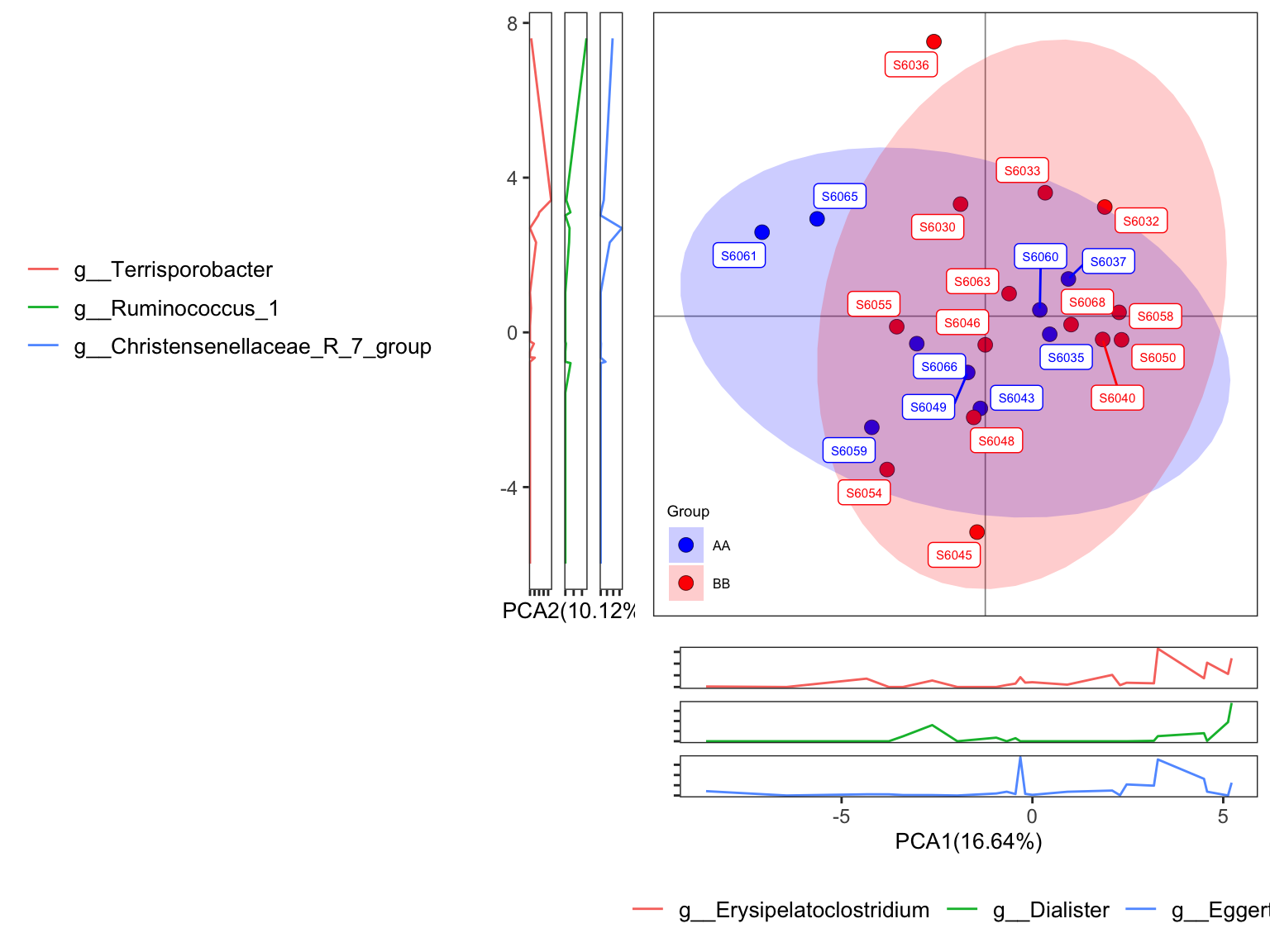
Figure 11.26: plot_Ordination (ellipse with 95% confidence interval)
- ellipse with groups
plot_Ordination(ResultList = ordination_PCA,
                group = "Group",
                group_names = c("AA", "BB"),
                group_color = c("blue", "red"),
                circle_type = "ellipse_groups",
                sample = TRUE)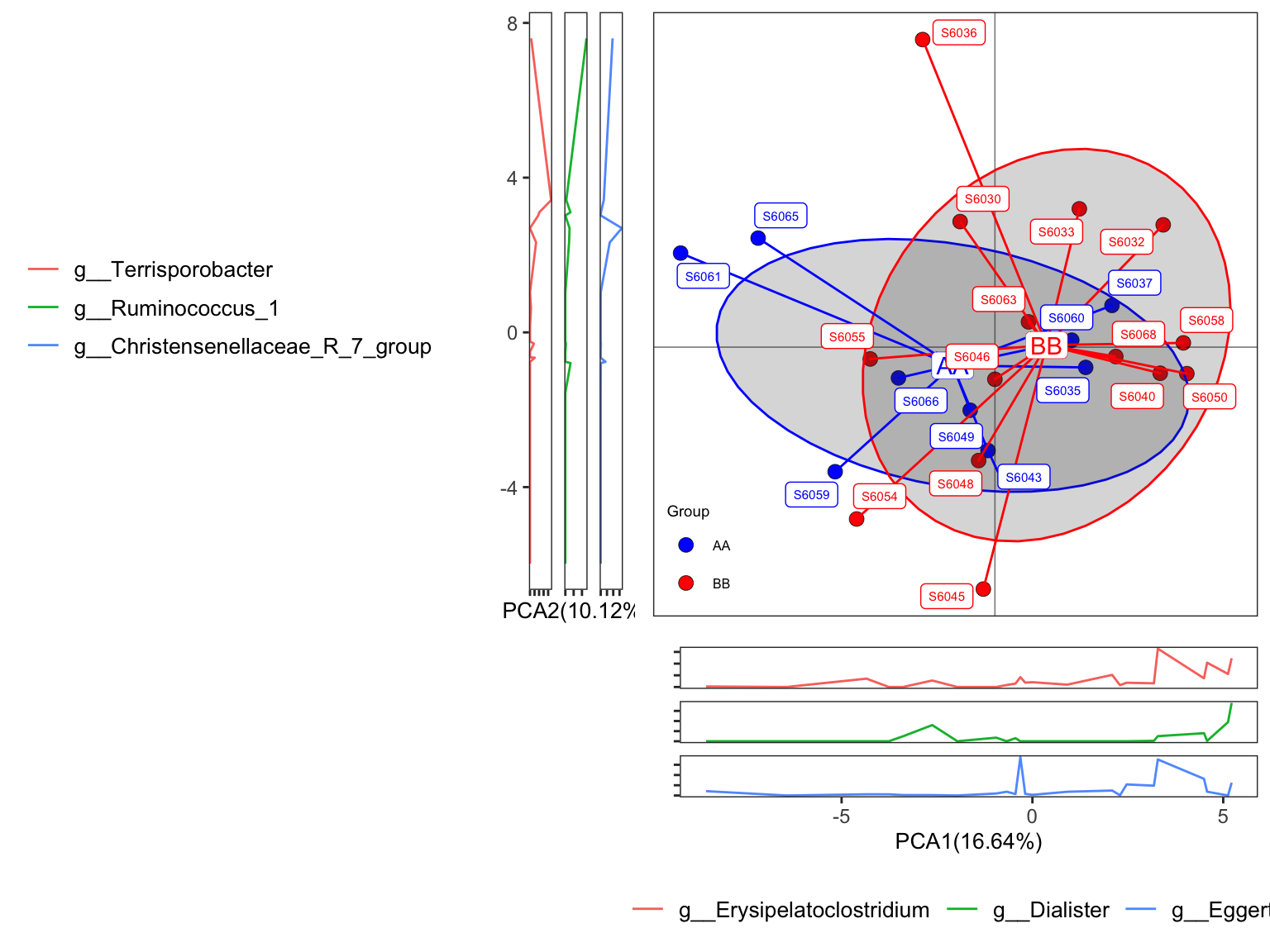
Figure 11.27: plot_Ordination (ellipse with groups)
- ellipse with border line
plot_Ordination(ResultList = ordination_PCA,
                group = "Group",
                group_names = c("AA", "BB"),
                group_color = c("blue", "red"),
                circle_type = "ellipse_line",
                sample = TRUE)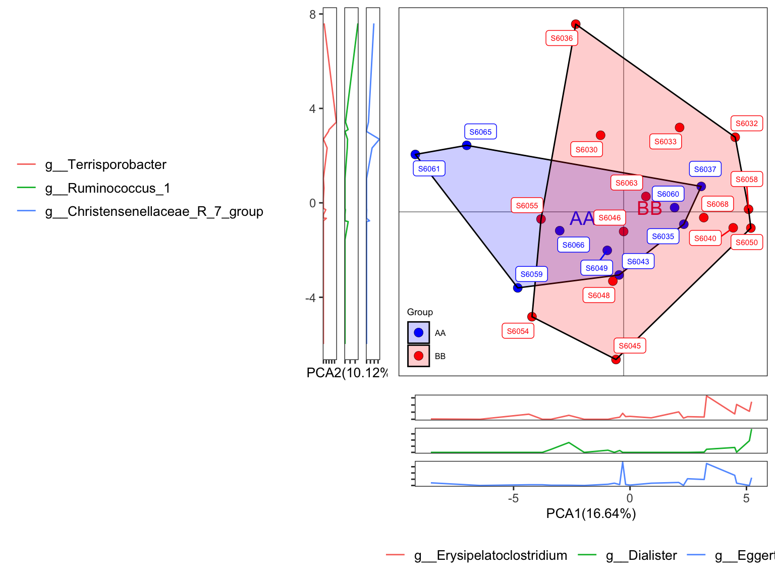
Figure 11.28: plot_Ordination (ellipse with border line)
- plot with SampleID and sideboxplot and setting group colors
plot_Ordination(ResultList = ordination_PCA,
                group = "Group",
                group_names = c("AA", "BB"),
                group_color = c("blue", "red"),
                circle_type = "ellipse",
                sidelinechart = FALSE,
                sideboxplot = TRUE,
                sample = TRUE)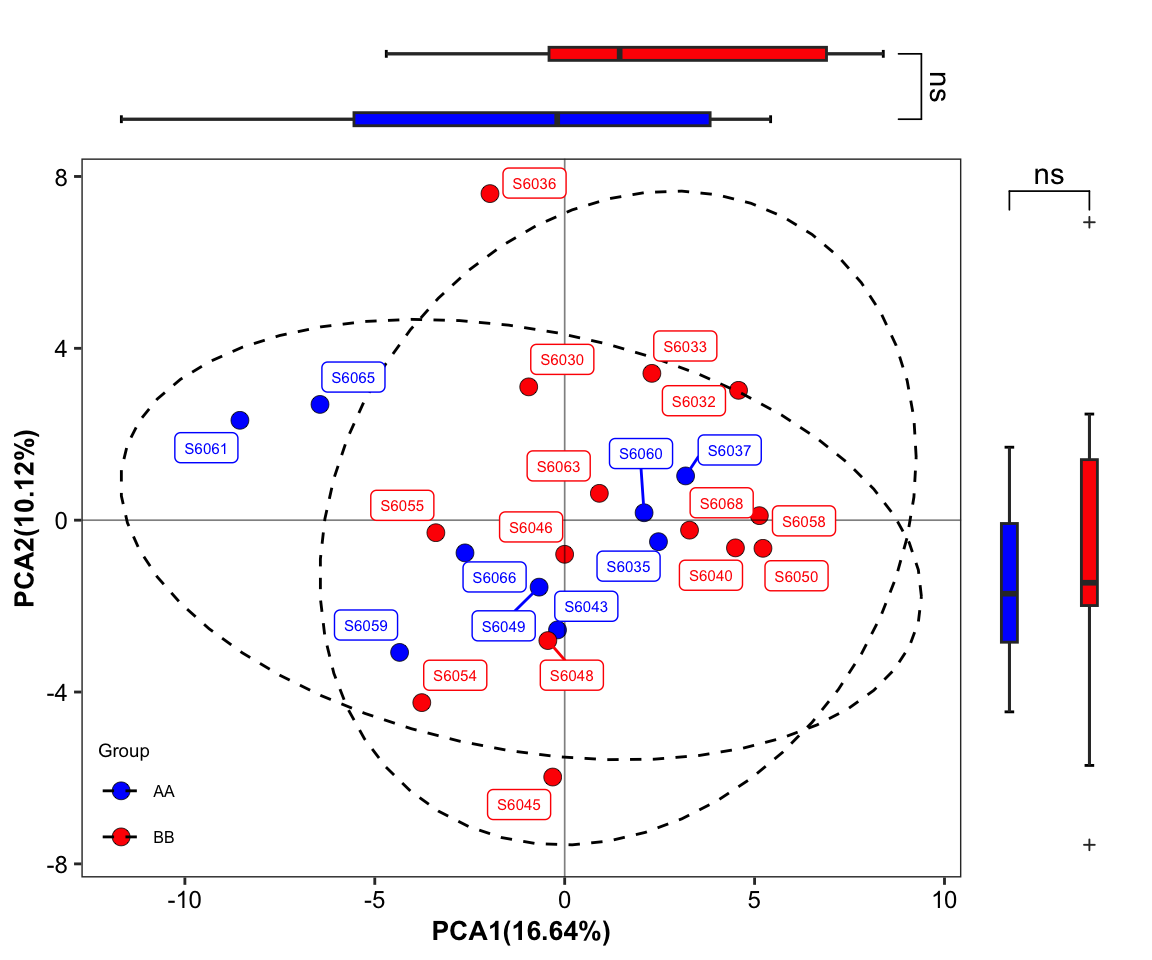
Figure 11.29: plot_Ordination (Ordinary pattern with SampleID sideboxplot)
- plot with SampleID and sideboxplot and setting group colors 2
plot_Ordination(ResultList = ordination_PCA,
                group = "Group",
                group_names = c("AA", "BB"),
                group_color = c("blue", "red"),
                circle_type = "ellipse_CI",
                sidelinechart = FALSE,
                sideboxplot = TRUE,
                sample = TRUE)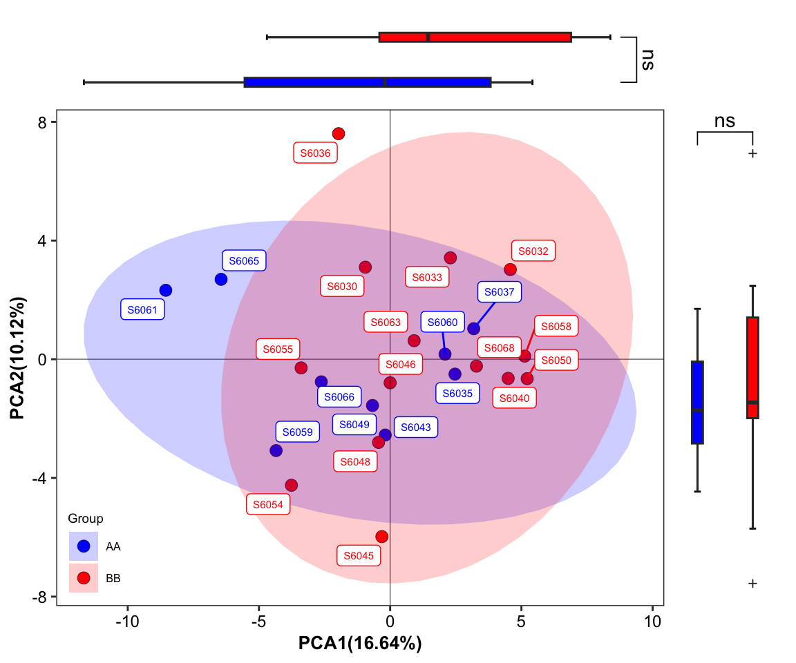
Figure 11.30: plot_Ordination (ellipse_CI with SampleID sideboxplot)
- plot with SampleID and sideboxplot and setting group colors 3
plot_Ordination(ResultList = ordination_PCA,
                group = "Group",
                group_names = c("AA", "BB"),
                group_color = c("blue", "red"),
                circle_type = "ellipse_groups",
                sidelinechart = FALSE,
                sideboxplot = TRUE,
                sample = TRUE)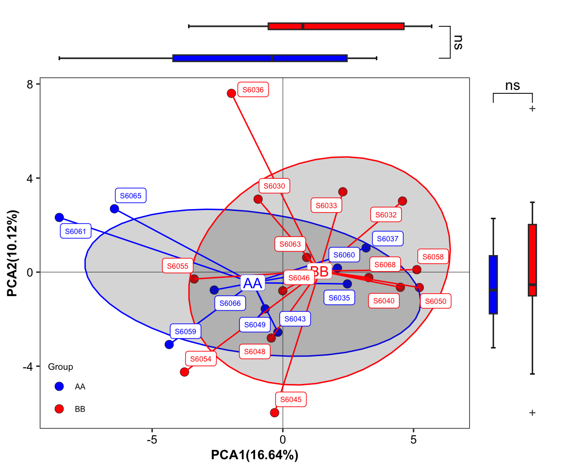
Figure 11.31: plot_Ordination (ellipse_groups with SampleID sideboxplot)
- plot with SampleID and sideboxplot and setting group colors 4
plot_Ordination(ResultList = ordination_PCA,
                group = "Group",
                group_names = c("AA", "BB"),
                group_color = c("blue", "red"),
                circle_type = "ellipse_line",
                sidelinechart = FALSE,
                sideboxplot = TRUE,
                sample = TRUE)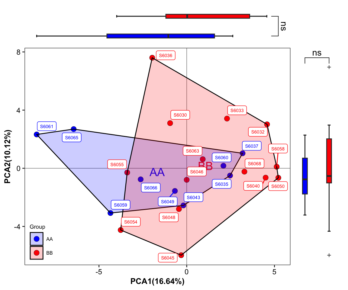
Figure 11.32: plot_Ordination (ellipse_line with SampleID sideboxplot)
- plot with SampleID and sideboxplot and setting group colors and shape
data("amplicon_ps")
amplicon_ps_genus <- summarize_taxa(ps = amplicon_ps,
                                    taxa_level = "Genus")
amplicon_res_ordination <- run_ordination(
                              ps = amplicon_ps_genus,
                              group = "SampleType",
                              method = "PCoA")
## [1] "Pvalue of beta dispersion less than 0.05"plot_Ordination(ResultList = amplicon_res_ordination,
group = "SampleType",
shape_column = "ReportedAntibioticUsage",
shape_values = c(16, 17),
circle_type = "ellipse_line",
sidelinechart = FALSE,
sideboxplot = TRUE,
sample = TRUE)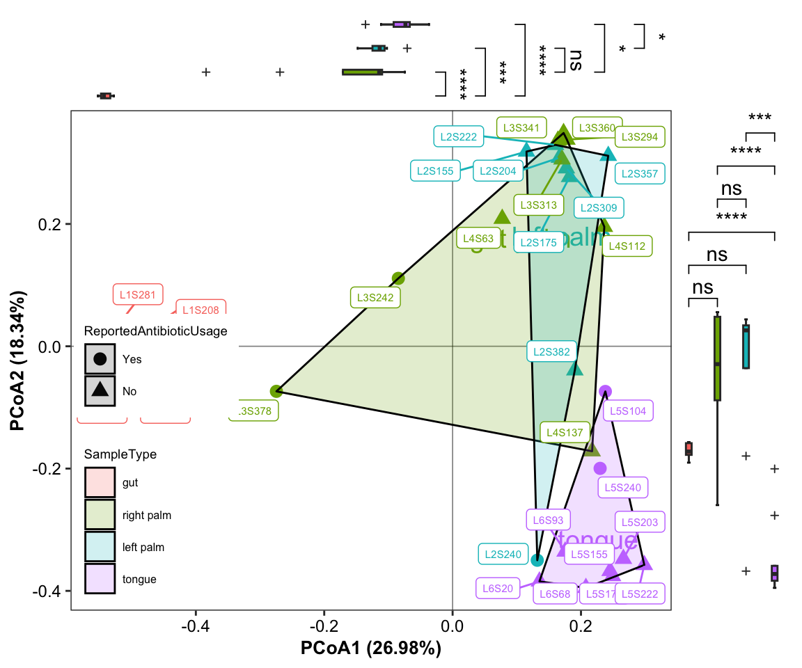
Figure 11.33: plot_Ordination (ellipse_line with SampleID sideboxplot)
11.9 plot_ggbiplot
- biplot with topN dominant taxa
plot_ggbiplot(ResultList = ordination_PCA,
              group = "Group",
              group_color = c("blue", "red"),
              topN = 5,
              ellipse = TRUE,
              labels = "SampleID")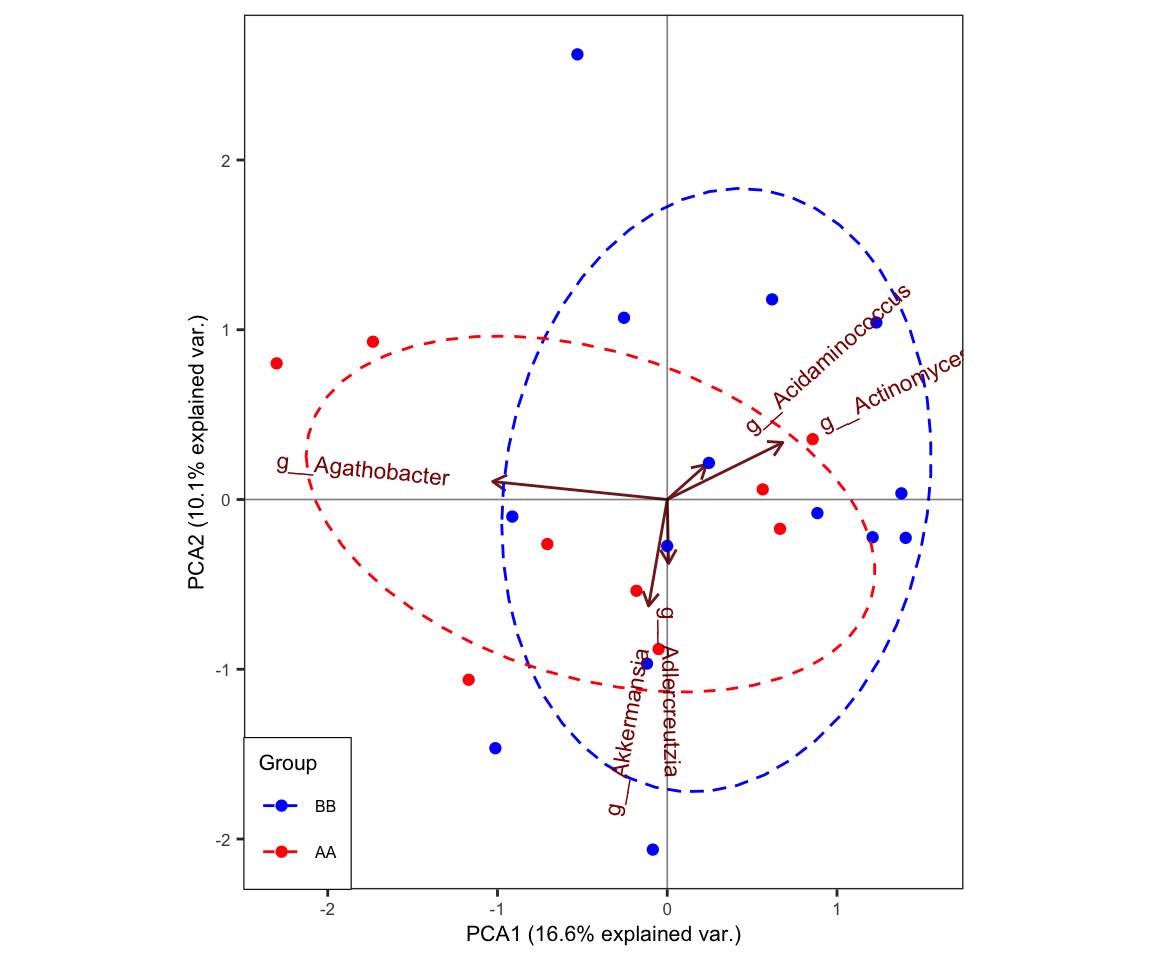
Figure 11.34: plot_ggbiplot (biplot)
11.10 plot_corrplot
dada2_beta <- run_beta_diversity(ps = dada2_ps_rarefy,
                                 method = "bray")
plot_distance_corrplot(datMatrix = dada2_beta$BetaDistance)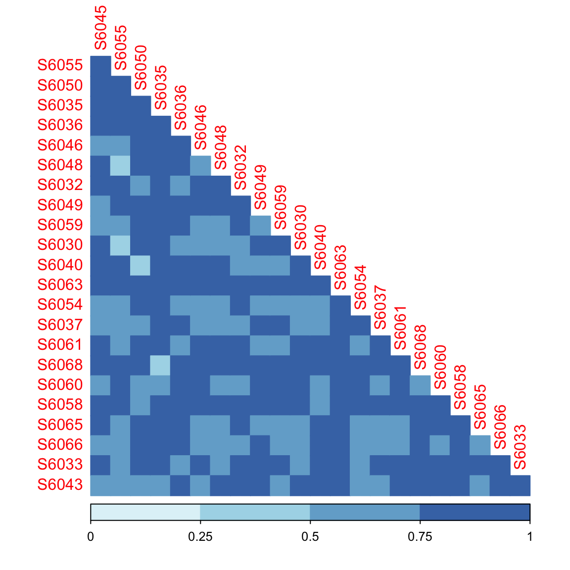
Figure 11.35: plot_corrplot (distance)
11.11 plot_2DA_venn
da_wilcox <- run_wilcox(
                ps = dada2_ps_genus_filter_trim,
                group = "Group",
                group_names = c("AA", "BB"))

da_ttest <- run_ttest(
               ps = dada2_ps_genus_filter_trim,
               group = "Group",
               group_names = c("AA", "BB"))

DA_venn_res <- plot_2DA_venn(
                   daTest1 = da_wilcox,
                   daTest2 = da_ttest,
                   datType1 = "AA vs BB(wilcox)",
                   datType2 = "AA vs BB(t-test)",
                   group_names = c("AA", "BB"),
                   Pvalue_name = "Pvalue",
                   logFc_name1 = "Log2FoldChange (Rank)\nAA_vs_BB",
                   logFc_name2 = "Log2FoldChange (Mean)\nAA_vs_BB",
                   Pvalue_cutoff = 0.8,
                   logFC_cutoff = 0.2)
DA_venn_res$pl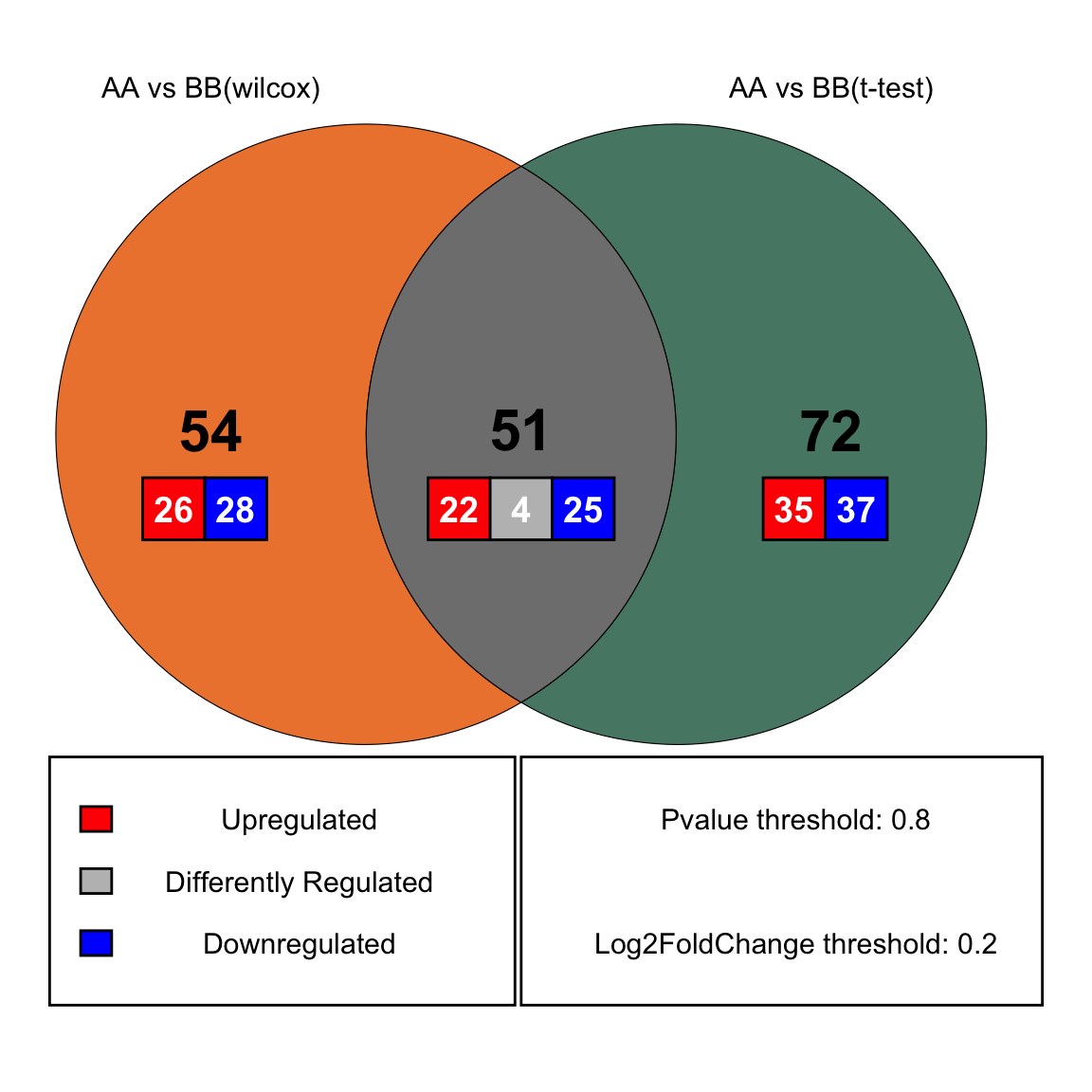
Figure 11.36: plot_2DA_venn (wilcox vs t_test)
11.12 plot the DA results from the significant taxa by double barplot
data("amplicon_ps")
DA_res <- run_wilcox(
              ps = amplicon_ps,
              taxa_level = "Family",
              group = "SampleType",
              group_names = c("tongue", "gut"))

plot_double_barplot(data = DA_res,
              x_index = "Log2FoldChange (Rank)\ntongue_vs_gut",
              x_index_cutoff = 1,
              y_index = "AdjustedPvalue",
              y_index_cutoff = 0.05)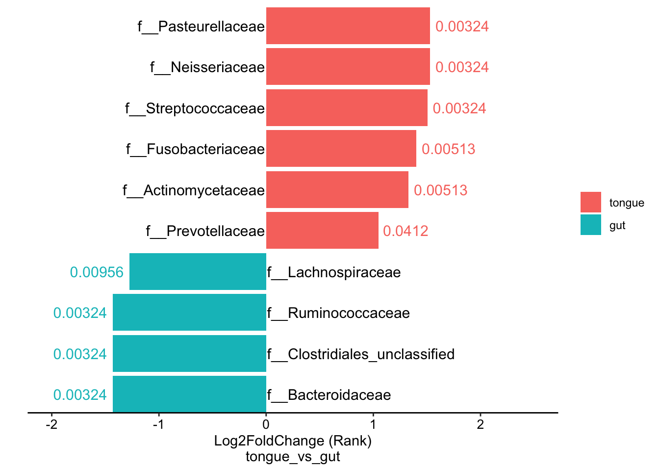
Figure 11.37: double barplot for DA results
11.13 plot_stacked_bar_XIVZ
- Minimum usage: plot in relative abundance
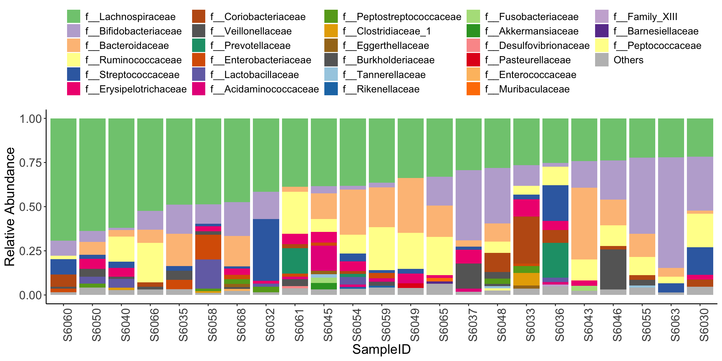
Figure 11.38: plot_stacked_bar_XIVZ (test1)
- Set feature parameter to show feature information
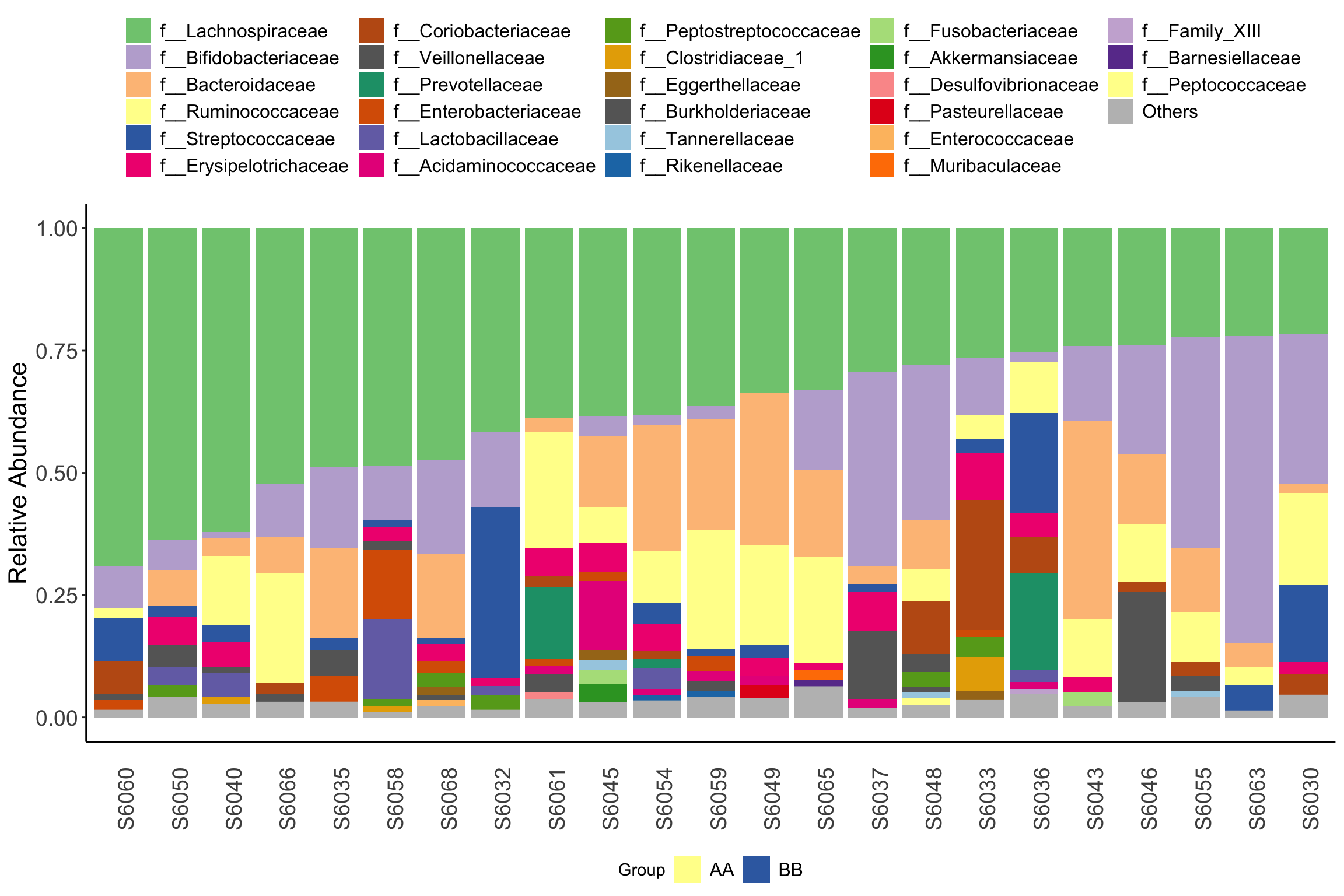
Figure 11.39: plot_stacked_bar_XIVZ (test2)
- Pass ordered sample names to order parameter to plot in specific order
metadata <- phyloseq::sample_data(dada2_ps_rarefy) %>%
  data.frame() %>%
  dplyr::arrange(Group)
plot_stacked_bar_XIVZ(phyloseq = dada2_ps_rarefy,
                 level = "Family",
                 feature = "Group",
                 order = rownames(metadata))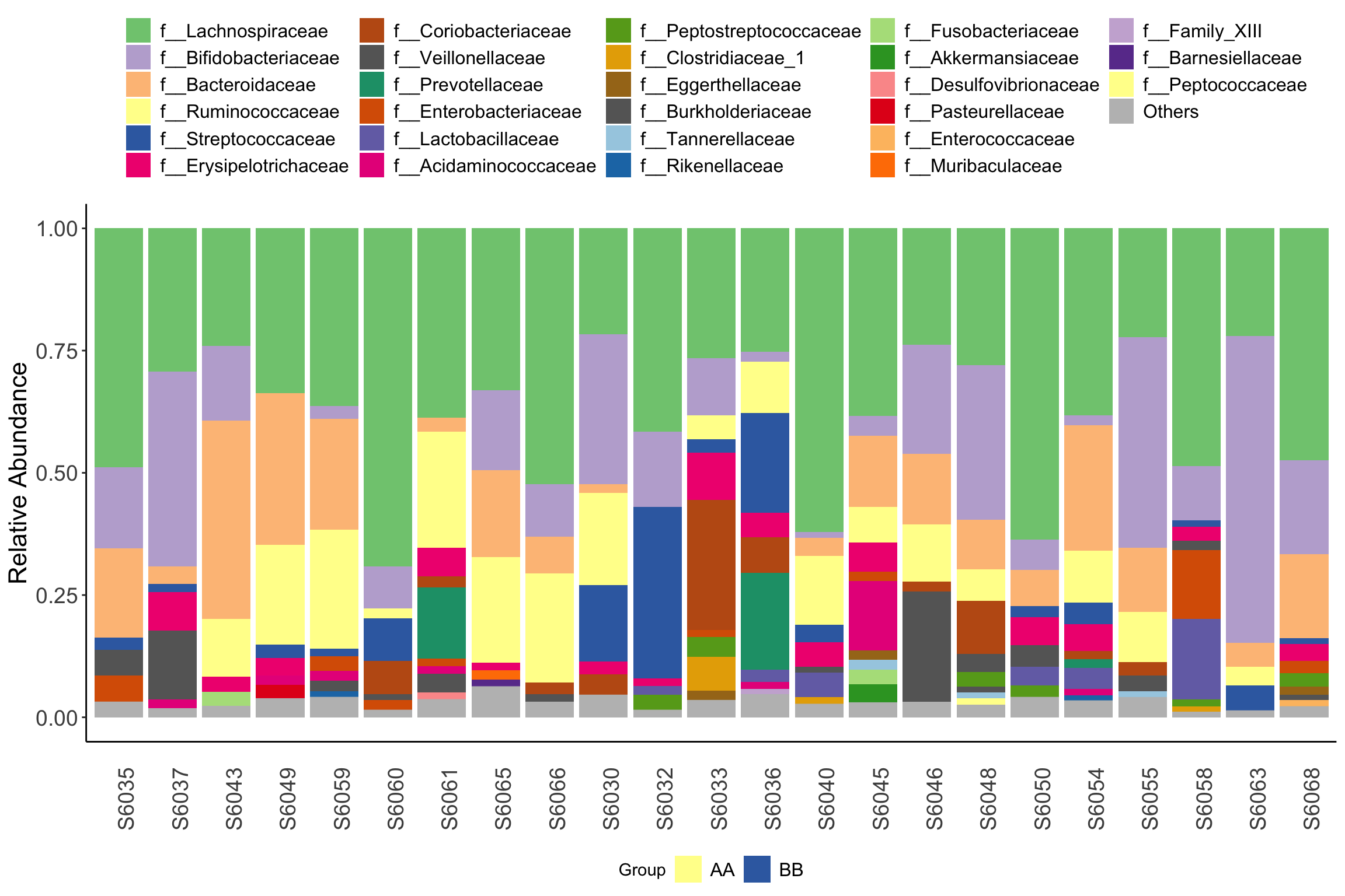
Figure 11.40: plot_stacked_bar_XIVZ (test3)
- Use facet_wrap(vars(), scale=“free”) funciton to facet stacked barplot
plot_stacked_bar_XIVZ(phyloseq = dada2_ps_rarefy,
                 level = "Family",
                 relative_abundance = TRUE,
                 order = rownames(metadata)) +
  facet_wrap(vars(Group), scale="free")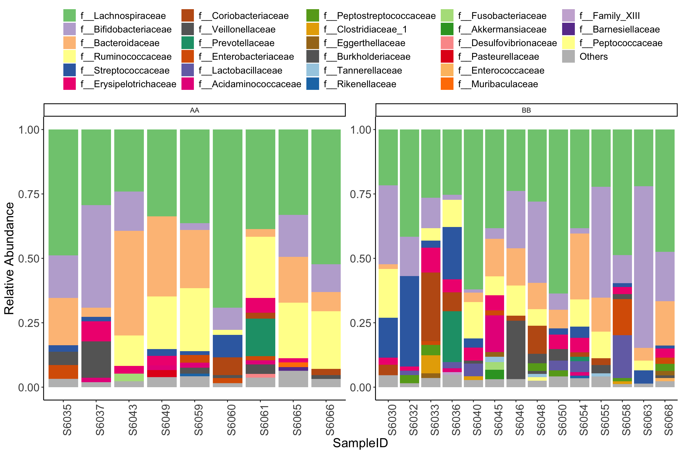
Figure 11.41: plot_stacked_bar_XIVZ (test4)
11.14 plot_StackBarPlot
plot_StackBarPlot provides too many parameters for users to display the Stacked barplot of microbial composition by using ggplot2 format. Here is the ordinary pattern. More details to see help(plot_StackBarPlot).
- Ordinary pattern
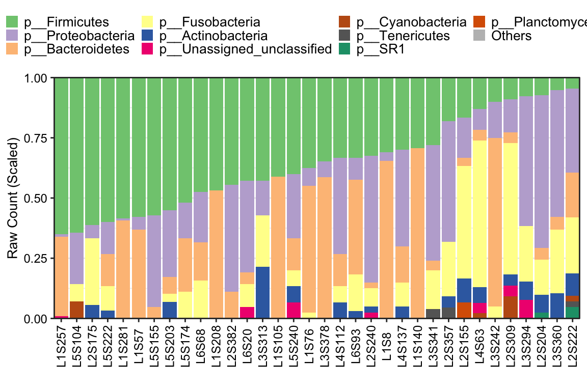
Figure 11.42: plot_StackBarPlot(Ordinary pattern)
- Metadata with
SampleTypephenotype
## [1] "This palatte have 20 colors!"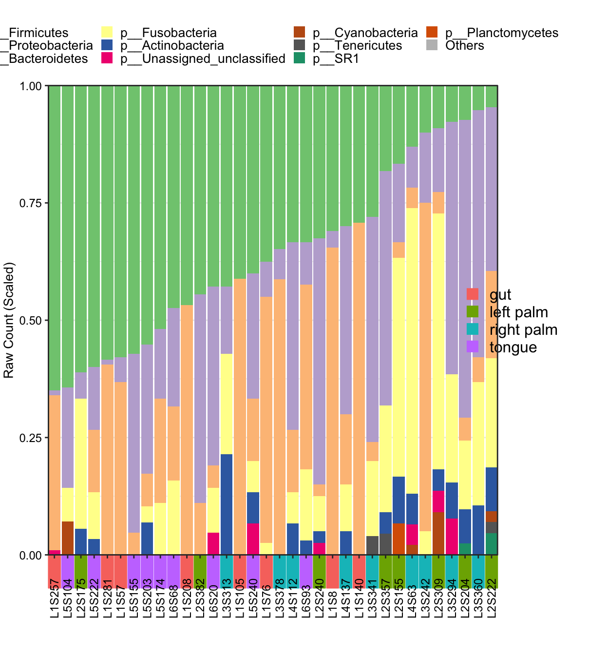
Figure 11.43: plot_StackBarPlot (Metadata with group)
- Metadata with
SampleTypephenotype in cluster mode
plot_StackBarPlot(
        ps = amplicon_ps_rarefy,
        taxa_level = "Phylum",
        group = "SampleType",
        cluster = TRUE)
## [1] "This palatte have 20 colors!"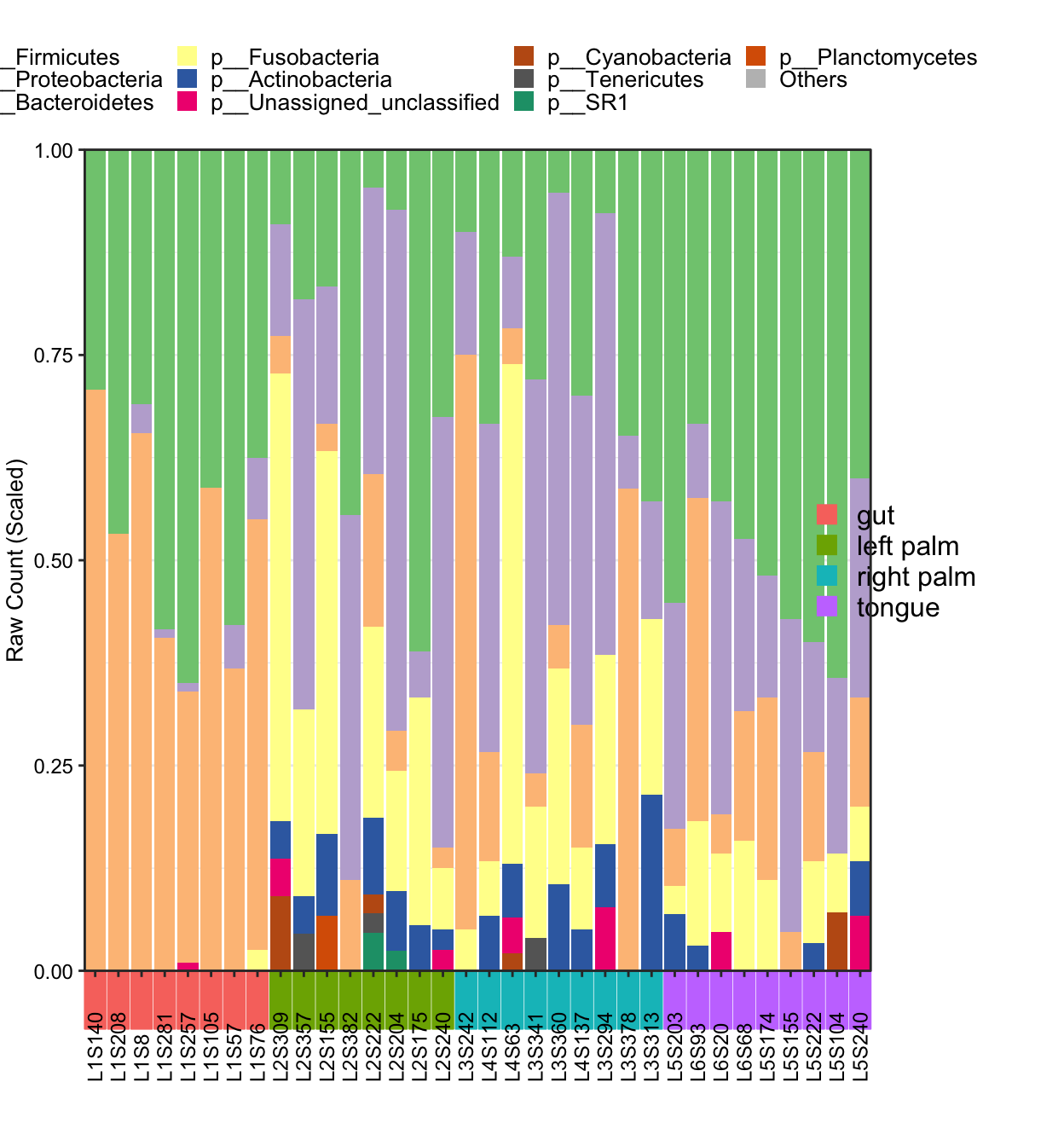
Figure 11.44: plot_StackBarPlot (Metadata with group in cluster mode)
- Metadata with
SampleTypephenotype in facet
plot_StackBarPlot(
        ps = amplicon_ps_rarefy,
        taxa_level = "Phylum",
        group = "SampleType",
        facet = TRUE)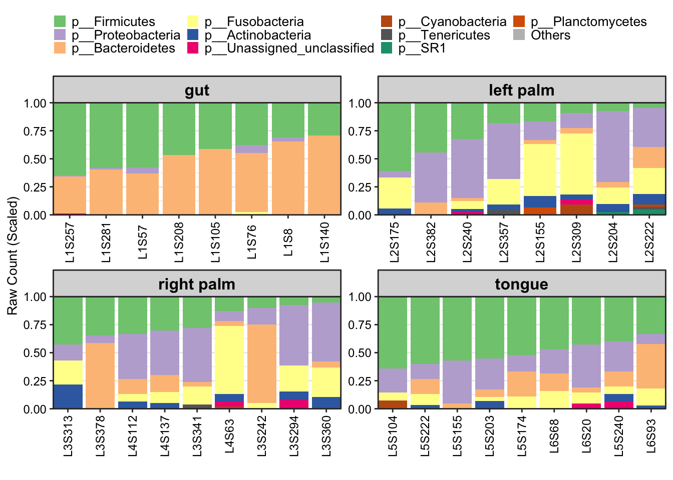
Figure 11.45: plot_StackBarPlot (Metadata with group in facet)
- Metadata with two groups to display samples
plot_StackBarPlot(
  ps = amplicon_ps_rarefy,
  taxa_level = "Order",
  group = "SampleType",
  subgroup = "Year")
## [1] "This palatte have 19 colors!"
## [1] "This palatte have 20 colors!"
## [1] "This palatte have 20 colors!"
## [1] "This palatte have 20 colors!"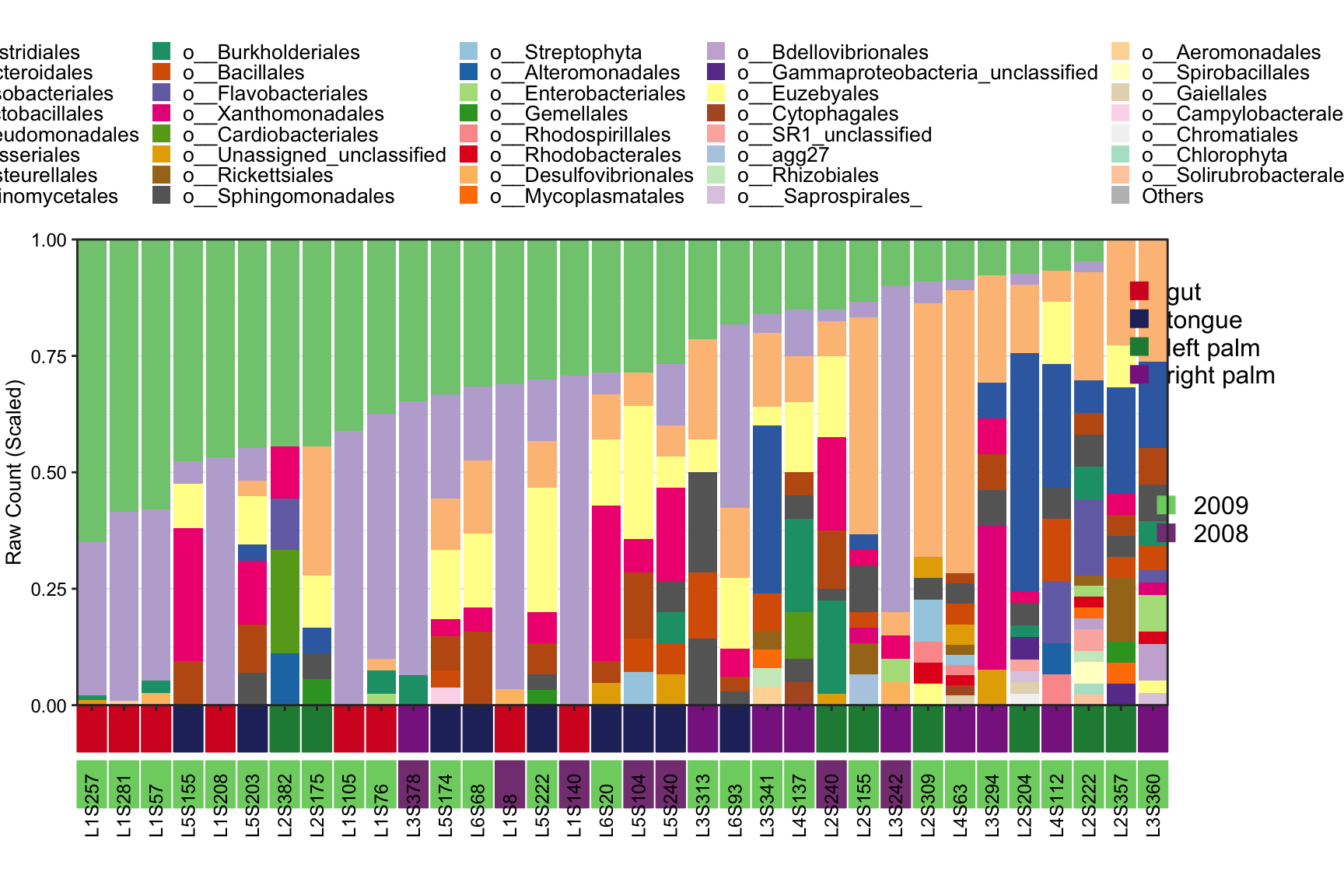
Figure 11.46: plot_StackBarPlot (Metadata with two groups ot display samples)
- Metadata with three groups to display samples
plot_StackBarPlot(
  ps = amplicon_ps_rarefy,
  taxa_level = "Order",
  group = "SampleType",
  subgroup = c("Year", "Month"))
## [1] "This palatte have 19 colors!"
## [1] "This palatte have 20 colors!"
## [1] "This palatte have 20 colors!"
## [1] "This palatte have 20 colors!"
## [1] "This palatte have 20 colors!"
## [1] "This palatte have 20 colors!"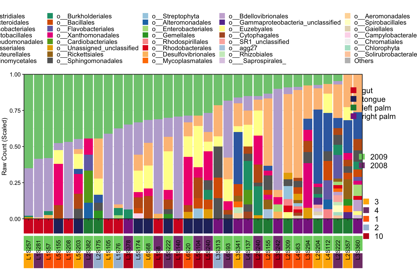
Figure 11.47: plot_StackBarPlot (Metadata with three groups ot display samples)
- Order SampleID by orderSample parameter
plot_StackBarPlot(
  ps = amplicon_ps_rarefy,
  taxa_level = "Order",
  group = "SampleType",
  orderSample = phyloseq::sample_names(amplicon_ps)[1:10])
## [1] "This palatte have 20 colors!"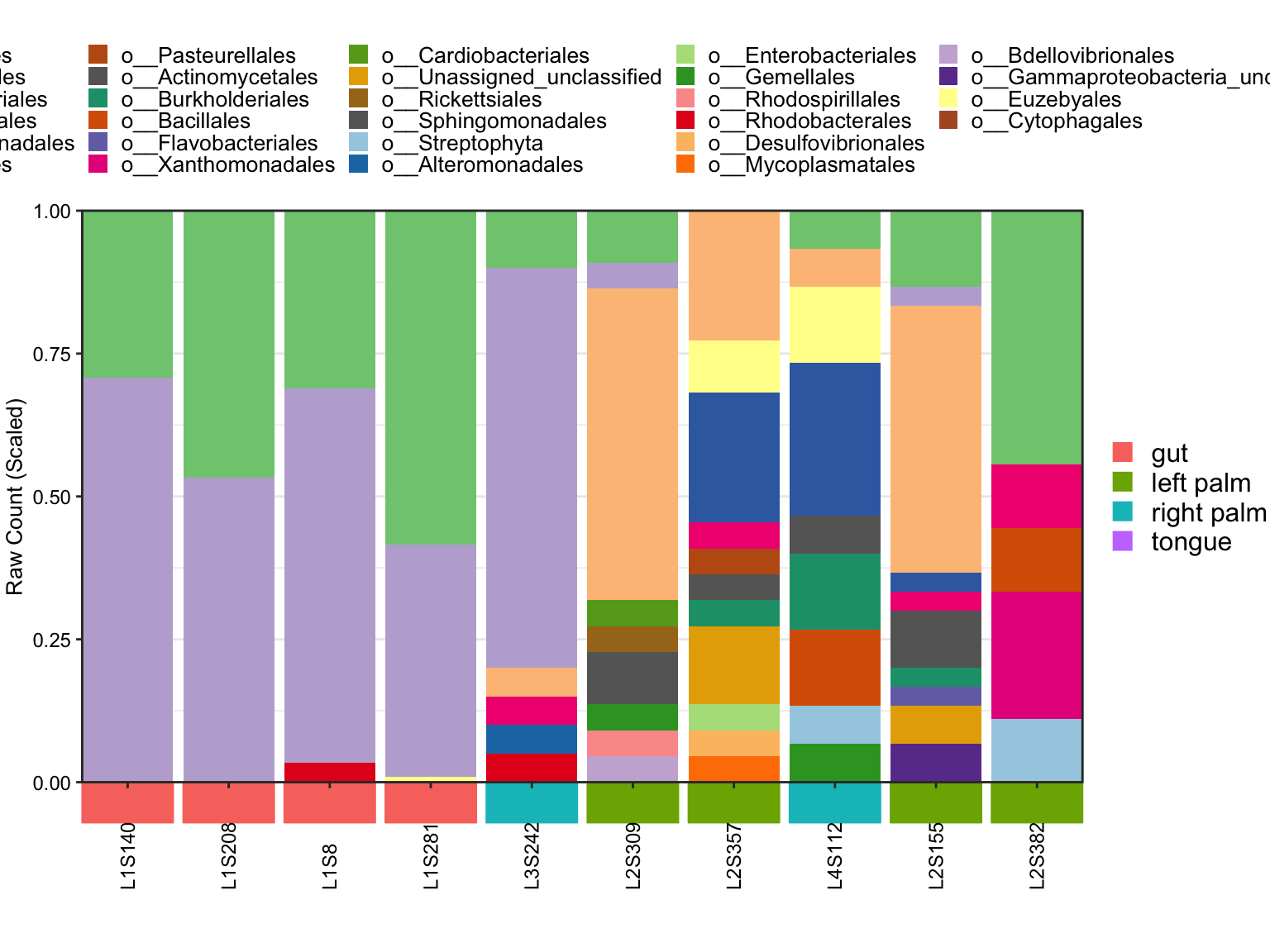
Figure 11.48: Stacked barplot with Ordered Samples
- Hide sample names by sample_label parameter
plot_StackBarPlot(
  ps = amplicon_ps_rarefy,
  taxa_level = "Order",
  group = "SampleType",
  orderSample = phyloseq::sample_names(amplicon_ps)[1:10],
  sample_label = FALSE)
## [1] "This palatte have 20 colors!"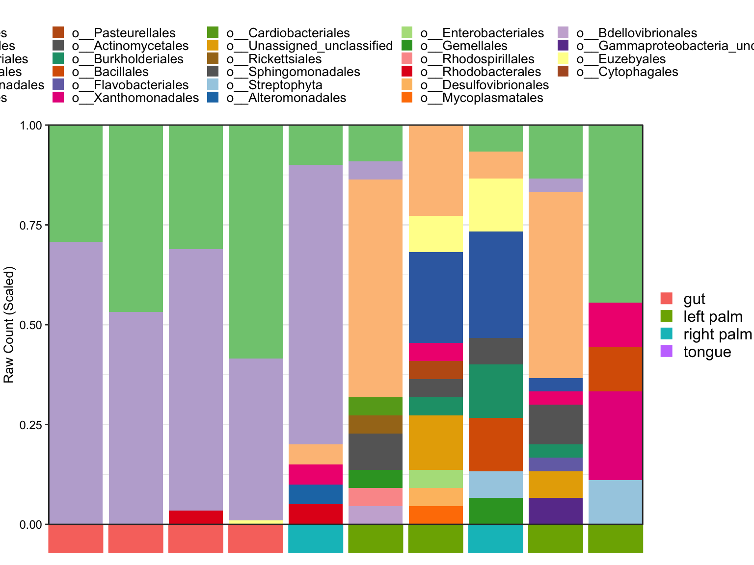
Figure 11.49: Stacked barplot with hiding Samples’ names
11.15 Color Palettes
11.15.1 Wes Anderson Palettes
Wes Anderson Palettes is from wesanderson package and we have integrated it into XMAS2.0.
data("amplicon_ps")
dat_alpha <- run_alpha_diversity(ps = amplicon_ps, measures = c("Shannon", "Chao1"))
# origin
pl_origin <- plot_boxplot(data = dat_alpha,
y_index = "Shannon",
group = "SampleType",
do_test = TRUE,
cmp_list = list(c("gut", "right palm"), c("gut", "left palm")),
method = "wilcox.test")
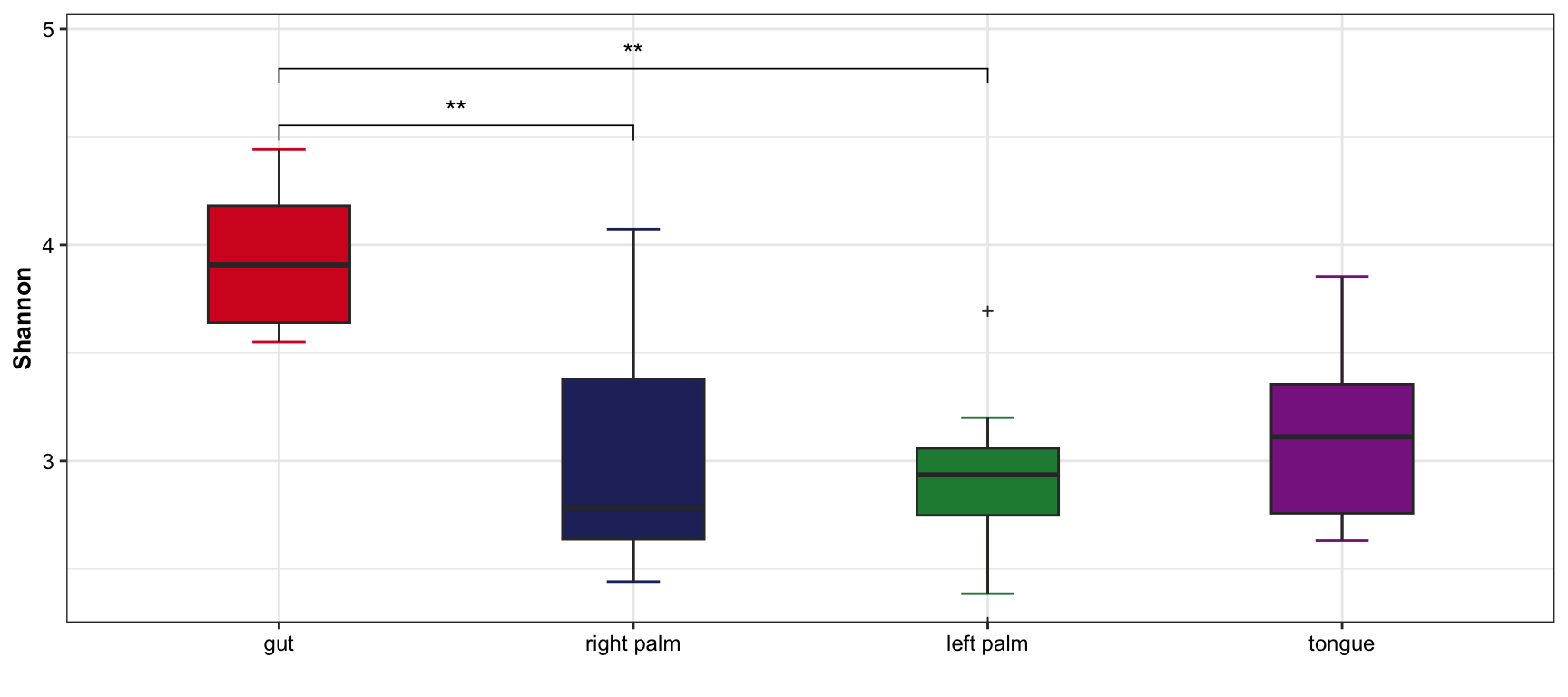
# Wes Anderson Palettes
pal <- wes_palette(name = "GrandBudapest1", 4, type = "discrete")
pl_wes <- plot_boxplot(data = dat_alpha,
y_index = "Shannon",
group = "SampleType",
group_color = pal,
do_test = TRUE,
cmp_list = list(c("gut", "right palm"), c("gut", "left palm")),
method = "wilcox.test")
cowplot::plot_grid(pl_origin, pl_wes,
align = "hv",
labels = c("Origin", "Wes Anderson"))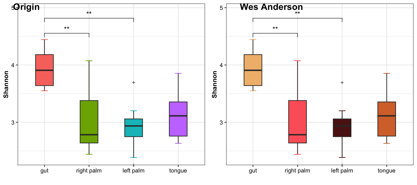
Figure 11.50: Wes Anderson Palettes
11.16 Ordination plots with ggplot2
11.16.1 principal components analysis with the iris data set
ord <- prcomp(iris[, 1:4])

ggord(ord, iris$Species, cols = c('purple', 'orange', 'blue')) +
  scale_shape_manual('Groups', values = c(1, 2, 3)) +
  theme_classic() +
  theme(legend.position = 'top')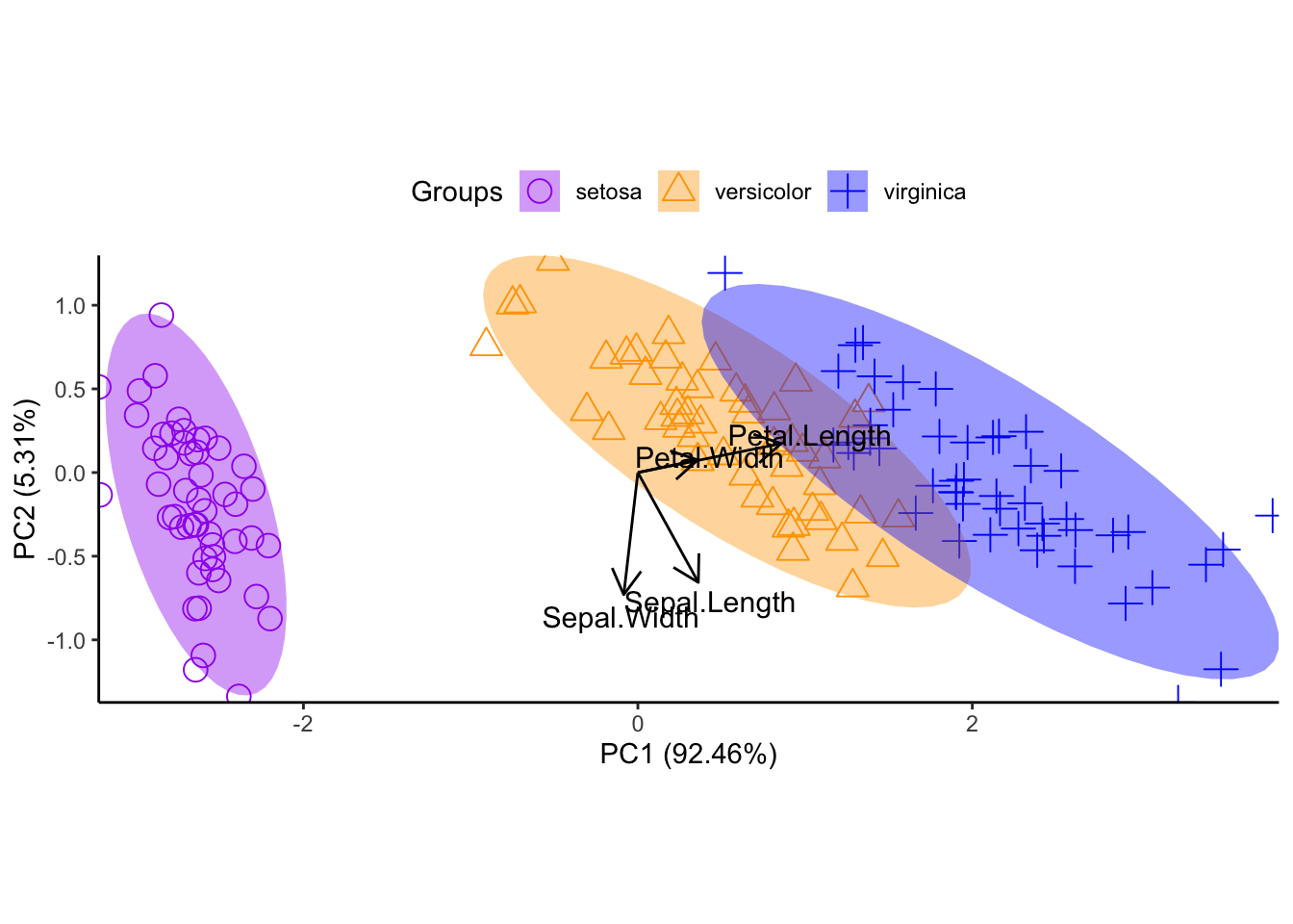
Figure 11.52: principal components analysis
11.16.2 multiple correspondence analysis with the tea dataset
data(tea, package = 'FactoMineR')
tea <- tea[, c('Tea', 'sugar', 'price', 'age_Q', 'sex')]

ord <- FactoMineR::MCA(tea[, -1], graph = FALSE)

ggord(ord, tea$Tea, parse = FALSE) # use parse = FALSE for labels with non alphanumeric characters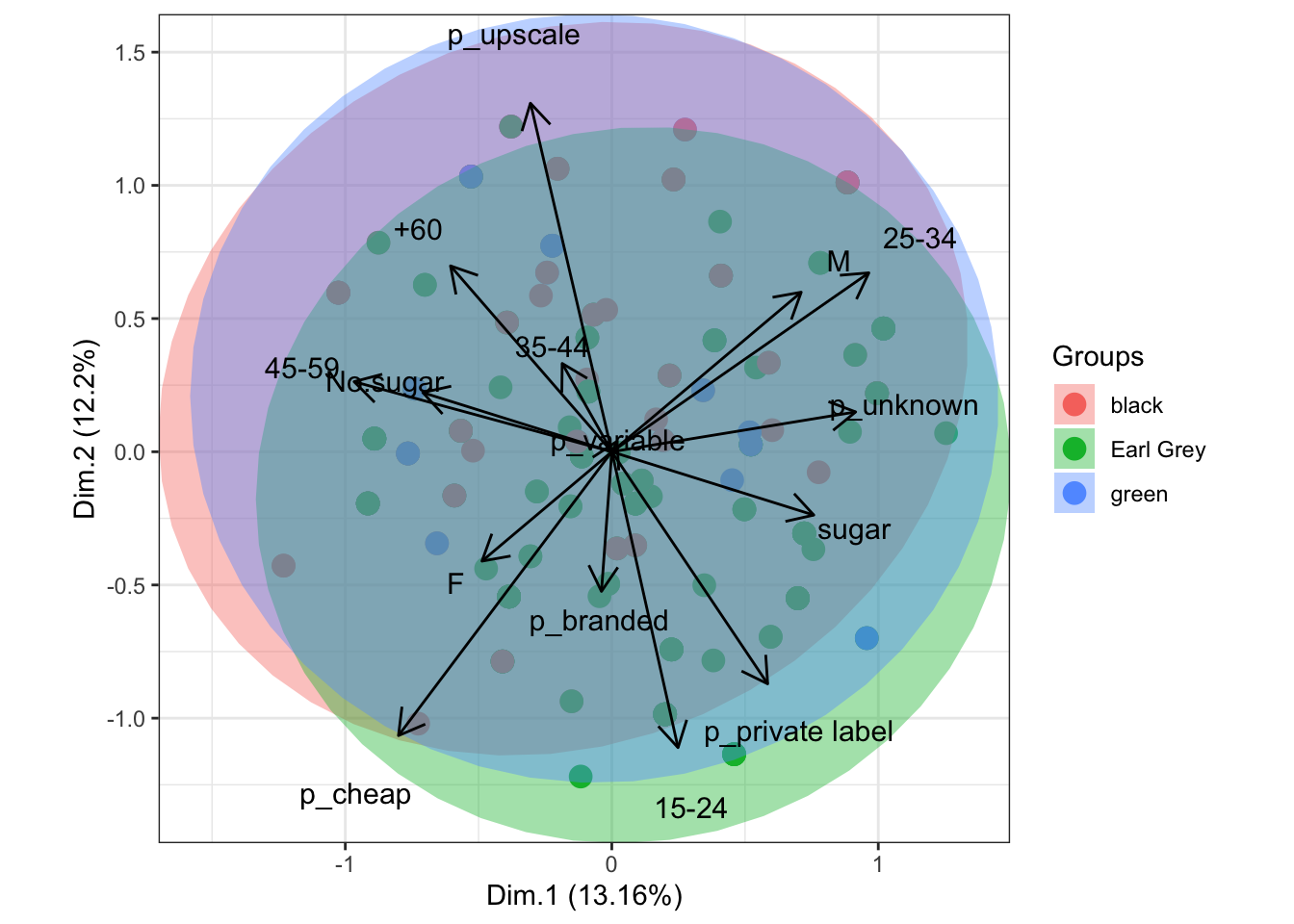
Figure 11.53: multiple correspondence analysis
11.17 Systematic Information
## ─ Session info ───────────────────────────────────────────────────────────────────────────────────────────────────────────────────────────
##  setting  value
##  version  R version 4.1.3 (2022-03-10)
##  os       macOS Monterey 12.2.1
##  system   x86_64, darwin17.0
##  ui       RStudio
##  language (EN)
##  collate  en_US.UTF-8
##  ctype    en_US.UTF-8
##  tz       Asia/Shanghai
##  date     2023-11-30
##  rstudio  2023.09.0+463 Desert Sunflower (desktop)
##  pandoc   3.1.1 @ /Applications/RStudio.app/Contents/Resources/app/quarto/bin/tools/ (via rmarkdown)
##
## ─ Packages ───────────────────────────────────────────────────────────────────────────────────────────────────────────────────────────────
##  package              * version   date (UTC) lib source
##  abind                  1.4-5     2016-07-21 [2] CRAN (R 4.1.0)
##  ade4                   1.7-22    2023-02-06 [2] CRAN (R 4.1.2)
##  ALDEx2                 1.30.0    2022-11-01 [2] Bioconductor
##  annotate               1.72.0    2021-10-26 [2] Bioconductor
##  AnnotationDbi          1.60.2    2023-03-10 [2] Bioconductor
##  ape                  * 5.7-1     2023-03-13 [2] CRAN (R 4.1.2)
##  askpass                1.1       2019-01-13 [2] CRAN (R 4.1.0)
##  backports              1.4.1     2021-12-13 [2] CRAN (R 4.1.0)
##  base64enc              0.1-3     2015-07-28 [2] CRAN (R 4.1.0)
##  bayesm                 3.1-5     2022-12-02 [2] CRAN (R 4.1.2)
##  Biobase                2.54.0    2021-10-26 [2] Bioconductor
##  BiocGenerics           0.40.0    2021-10-26 [2] Bioconductor
##  BiocParallel           1.28.3    2021-12-09 [2] Bioconductor
##  biomformat             1.22.0    2021-10-26 [2] Bioconductor
##  Biostrings             2.62.0    2021-10-26 [2] Bioconductor
##  bit                    4.0.5     2022-11-15 [2] CRAN (R 4.1.2)
##  bit64                  4.0.5     2020-08-30 [2] CRAN (R 4.1.0)
##  bitops                 1.0-7     2021-04-24 [2] CRAN (R 4.1.0)
##  blob                   1.2.4     2023-03-17 [2] CRAN (R 4.1.2)
##  bookdown               0.34      2023-05-09 [2] CRAN (R 4.1.2)
##  broom                  1.0.5     2023-06-09 [2] CRAN (R 4.1.3)
##  bslib                  0.6.0     2023-11-21 [1] CRAN (R 4.1.3)
##  cachem                 1.0.8     2023-05-01 [2] CRAN (R 4.1.2)
##  callr                  3.7.3     2022-11-02 [2] CRAN (R 4.1.2)
##  car                    3.1-2     2023-03-30 [2] CRAN (R 4.1.2)
##  carData                3.0-5     2022-01-06 [2] CRAN (R 4.1.2)
##  caTools                1.18.2    2021-03-28 [2] CRAN (R 4.1.0)
##  checkmate              2.2.0     2023-04-27 [2] CRAN (R 4.1.2)
##  class                  7.3-22    2023-05-03 [2] CRAN (R 4.1.2)
##  classInt               0.4-9     2023-02-28 [2] CRAN (R 4.1.2)
##  cli                    3.6.1     2023-03-23 [2] CRAN (R 4.1.2)
##  cluster                2.1.4     2022-08-22 [2] CRAN (R 4.1.2)
##  coda                   0.19-4    2020-09-30 [2] CRAN (R 4.1.0)
##  codetools              0.2-19    2023-02-01 [2] CRAN (R 4.1.2)
##  coin                   1.4-2     2021-10-08 [2] CRAN (R 4.1.0)
##  colorspace             2.1-0     2023-01-23 [2] CRAN (R 4.1.2)
##  compositions           2.0-6     2023-04-13 [2] CRAN (R 4.1.2)
##  conflicted           * 1.2.0     2023-02-01 [2] CRAN (R 4.1.2)
##  corrplot               0.92      2021-11-18 [2] CRAN (R 4.1.0)
##  cowplot                1.1.1     2020-12-30 [2] CRAN (R 4.1.0)
##  crayon                 1.5.2     2022-09-29 [2] CRAN (R 4.1.2)
##  crosstalk              1.2.0     2021-11-04 [2] CRAN (R 4.1.0)
##  data.table             1.14.8    2023-02-17 [2] CRAN (R 4.1.2)
##  DBI                    1.1.3     2022-06-18 [2] CRAN (R 4.1.2)
##  DelayedArray           0.20.0    2021-10-26 [2] Bioconductor
##  DEoptimR               1.0-14    2023-06-09 [2] CRAN (R 4.1.3)
##  DESeq2                 1.34.0    2021-10-26 [2] Bioconductor
##  devtools               2.4.5     2022-10-11 [2] CRAN (R 4.1.2)
##  digest                 0.6.33    2023-07-07 [1] CRAN (R 4.1.3)
##  dplyr                * 1.1.2     2023-04-20 [2] CRAN (R 4.1.2)
##  DT                     0.28      2023-05-18 [2] CRAN (R 4.1.3)
##  e1071                  1.7-13    2023-02-01 [2] CRAN (R 4.1.2)
##  edgeR                  3.36.0    2021-10-26 [2] Bioconductor
##  ellipsis               0.3.2     2021-04-29 [2] CRAN (R 4.1.0)
##  emmeans                1.8.7     2023-06-23 [1] CRAN (R 4.1.3)
##  estimability           1.4.1     2022-08-05 [2] CRAN (R 4.1.2)
##  evaluate               0.21      2023-05-05 [2] CRAN (R 4.1.2)
##  FactoMineR             2.8       2023-03-27 [2] CRAN (R 4.1.2)
##  fansi                  1.0.4     2023-01-22 [2] CRAN (R 4.1.2)
##  farver                 2.1.1     2022-07-06 [2] CRAN (R 4.1.2)
##  fastmap                1.1.1     2023-02-24 [2] CRAN (R 4.1.2)
##  flashClust             1.01-2    2012-08-21 [2] CRAN (R 4.1.0)
##  foreach                1.5.2     2022-02-02 [2] CRAN (R 4.1.2)
##  foreign                0.8-84    2022-12-06 [2] CRAN (R 4.1.2)
##  Formula                1.2-5     2023-02-24 [2] CRAN (R 4.1.2)
##  fs                     1.6.2     2023-04-25 [2] CRAN (R 4.1.2)
##  genefilter             1.76.0    2021-10-26 [2] Bioconductor
##  geneplotter            1.72.0    2021-10-26 [2] Bioconductor
##  generics               0.1.3     2022-07-05 [2] CRAN (R 4.1.2)
##  GenomeInfoDb           1.30.1    2022-01-30 [2] Bioconductor
##  GenomeInfoDbData       1.2.7     2022-03-09 [2] Bioconductor
##  GenomicRanges          1.46.1    2021-11-18 [2] Bioconductor
##  ggiraph                0.8.7     2023-03-17 [2] CRAN (R 4.1.2)
##  ggiraphExtra           0.3.0     2020-10-06 [2] CRAN (R 4.1.2)
##  ggplot2              * 3.4.2     2023-04-03 [2] CRAN (R 4.1.2)
##  ggpubr               * 0.6.0     2023-02-10 [2] CRAN (R 4.1.2)
##  ggrepel                0.9.3     2023-02-03 [2] CRAN (R 4.1.2)
##  ggsci                  3.0.0     2023-03-08 [2] CRAN (R 4.1.2)
##  ggsignif               0.6.4     2022-10-13 [2] CRAN (R 4.1.2)
##  ggVennDiagram          1.2.2     2022-09-08 [2] CRAN (R 4.1.2)
##  glmnet                 4.1-7     2023-03-23 [2] CRAN (R 4.1.2)
##  glue                   1.6.2     2022-02-24 [2] CRAN (R 4.1.2)
##  gplots                 3.1.3     2022-04-25 [2] CRAN (R 4.1.2)
##  gridExtra              2.3       2017-09-09 [2] CRAN (R 4.1.0)
##  gtable                 0.3.3     2023-03-21 [2] CRAN (R 4.1.2)
##  gtools                 3.9.4     2022-11-27 [2] CRAN (R 4.1.2)
##  highr                  0.10      2022-12-22 [2] CRAN (R 4.1.2)
##  Hmisc                  5.1-0     2023-05-08 [2] CRAN (R 4.1.2)
##  htmlTable              2.4.1     2022-07-07 [2] CRAN (R 4.1.2)
##  htmltools              0.5.7     2023-11-03 [1] CRAN (R 4.1.3)
##  htmlwidgets            1.6.2     2023-03-17 [2] CRAN (R 4.1.2)
##  httpuv                 1.6.11    2023-05-11 [2] CRAN (R 4.1.3)
##  httr                   1.4.6     2023-05-08 [2] CRAN (R 4.1.2)
##  igraph                 1.5.0     2023-06-16 [1] CRAN (R 4.1.3)
##  insight                0.19.3    2023-06-29 [2] CRAN (R 4.1.3)
##  IRanges                2.28.0    2021-10-26 [2] Bioconductor
##  iterators              1.0.14    2022-02-05 [2] CRAN (R 4.1.2)
##  jquerylib              0.1.4     2021-04-26 [2] CRAN (R 4.1.0)
##  jsonlite               1.8.7     2023-06-29 [2] CRAN (R 4.1.3)
##  kableExtra             1.3.4     2021-02-20 [2] CRAN (R 4.1.2)
##  KEGGREST               1.34.0    2021-10-26 [2] Bioconductor
##  KernSmooth             2.23-22   2023-07-10 [2] CRAN (R 4.1.3)
##  knitr                  1.43      2023-05-25 [2] CRAN (R 4.1.3)
##  labeling               0.4.2     2020-10-20 [2] CRAN (R 4.1.0)
##  later                  1.3.1     2023-05-02 [2] CRAN (R 4.1.2)
##  lattice              * 0.21-8    2023-04-05 [2] CRAN (R 4.1.2)
##  leaps                  3.1       2020-01-16 [2] CRAN (R 4.1.0)
##  libcoin                1.0-9     2021-09-27 [2] CRAN (R 4.1.0)
##  lifecycle              1.0.3     2022-10-07 [2] CRAN (R 4.1.2)
##  limma                  3.50.3    2022-04-07 [2] Bioconductor
##  locfit                 1.5-9.8   2023-06-11 [2] CRAN (R 4.1.3)
##  LOCOM                  1.1       2022-08-05 [2] Github (yijuanhu/LOCOM@c181e0f)
##  magrittr               2.0.3     2022-03-30 [2] CRAN (R 4.1.2)
##  MASS                   7.3-60    2023-05-04 [2] CRAN (R 4.1.2)
##  Matrix                 1.6-0     2023-07-08 [2] CRAN (R 4.1.3)
##  MatrixGenerics         1.6.0     2021-10-26 [2] Bioconductor
##  matrixStats            1.0.0     2023-06-02 [2] CRAN (R 4.1.3)
##  mbzinb                 0.2       2022-03-16 [2] local
##  memoise                2.0.1     2021-11-26 [2] CRAN (R 4.1.0)
##  metagenomeSeq          1.36.0    2021-10-26 [2] Bioconductor
##  mgcv                   1.8-42    2023-03-02 [2] CRAN (R 4.1.2)
##  microbiome             1.16.0    2021-10-26 [2] Bioconductor
##  mime                   0.12      2021-09-28 [2] CRAN (R 4.1.0)
##  miniUI                 0.1.1.1   2018-05-18 [2] CRAN (R 4.1.0)
##  modeltools             0.2-23    2020-03-05 [2] CRAN (R 4.1.0)
##  multcomp               1.4-25    2023-06-20 [2] CRAN (R 4.1.3)
##  multcompView           0.1-9     2023-04-09 [2] CRAN (R 4.1.2)
##  multtest               2.50.0    2021-10-26 [2] Bioconductor
##  munsell                0.5.0     2018-06-12 [2] CRAN (R 4.1.0)
##  mvtnorm                1.2-2     2023-06-08 [2] CRAN (R 4.1.3)
##  mycor                  0.1.1     2018-04-10 [2] CRAN (R 4.1.0)
##  NADA                   1.6-1.1   2020-03-22 [2] CRAN (R 4.1.0)
##  nlme                 * 3.1-162   2023-01-31 [2] CRAN (R 4.1.2)
##  nnet                   7.3-19    2023-05-03 [2] CRAN (R 4.1.2)
##  openssl                2.0.6     2023-03-09 [2] CRAN (R 4.1.2)
##  permute              * 0.9-7     2022-01-27 [2] CRAN (R 4.1.2)
##  pheatmap               1.0.12    2019-01-04 [2] CRAN (R 4.1.0)
##  phyloseq             * 1.38.0    2021-10-26 [2] Bioconductor
##  picante              * 1.8.2     2020-06-10 [2] CRAN (R 4.1.0)
##  pillar                 1.9.0     2023-03-22 [2] CRAN (R 4.1.2)
##  pkgbuild               1.4.2     2023-06-26 [2] CRAN (R 4.1.3)
##  pkgconfig              2.0.3     2019-09-22 [2] CRAN (R 4.1.0)
##  pkgload                1.3.2.1   2023-07-08 [2] CRAN (R 4.1.3)
##  plyr                   1.8.8     2022-11-11 [2] CRAN (R 4.1.2)
##  png                    0.1-8     2022-11-29 [2] CRAN (R 4.1.2)
##  ppcor                  1.1       2015-12-03 [2] CRAN (R 4.1.0)
##  prettyunits            1.1.1     2020-01-24 [2] CRAN (R 4.1.0)
##  processx               3.8.2     2023-06-30 [2] CRAN (R 4.1.3)
##  profvis                0.3.8     2023-05-02 [2] CRAN (R 4.1.2)
##  promises               1.2.0.1   2021-02-11 [2] CRAN (R 4.1.0)
##  protoclust             1.6.4     2022-04-01 [2] CRAN (R 4.1.2)
##  proxy                  0.4-27    2022-06-09 [2] CRAN (R 4.1.2)
##  ps                     1.7.5     2023-04-18 [2] CRAN (R 4.1.2)
##  pscl                   1.5.5.1   2023-05-10 [2] CRAN (R 4.1.2)
##  purrr                  1.0.1     2023-01-10 [2] CRAN (R 4.1.2)
##  qvalue                 2.26.0    2021-10-26 [2] Bioconductor
##  R6                     2.5.1     2021-08-19 [2] CRAN (R 4.1.0)
##  RAIDA                  1.0       2022-03-14 [2] local
##  RColorBrewer         * 1.1-3     2022-04-03 [2] CRAN (R 4.1.2)
##  Rcpp                   1.0.11    2023-07-06 [1] CRAN (R 4.1.3)
##  RcppZiggurat           0.1.6     2020-10-20 [2] CRAN (R 4.1.0)
##  RCurl                  1.98-1.12 2023-03-27 [2] CRAN (R 4.1.2)
##  remotes                2.4.2     2021-11-30 [2] CRAN (R 4.1.0)
##  reshape2               1.4.4     2020-04-09 [2] CRAN (R 4.1.0)
##  reticulate             1.30      2023-06-09 [2] CRAN (R 4.1.3)
##  Rfast                  2.0.8     2023-07-03 [2] CRAN (R 4.1.3)
##  rhdf5                  2.38.1    2022-03-10 [2] Bioconductor
##  rhdf5filters           1.6.0     2021-10-26 [2] Bioconductor
##  Rhdf5lib               1.16.0    2021-10-26 [2] Bioconductor
##  rlang                  1.1.1     2023-04-28 [1] CRAN (R 4.1.2)
##  rmarkdown              2.23      2023-07-01 [2] CRAN (R 4.1.3)
##  robustbase             0.99-0    2023-06-16 [2] CRAN (R 4.1.3)
##  rpart                  4.1.19    2022-10-21 [2] CRAN (R 4.1.2)
##  RSpectra               0.16-1    2022-04-24 [2] CRAN (R 4.1.2)
##  RSQLite                2.3.1     2023-04-03 [2] CRAN (R 4.1.2)
##  rstatix                0.7.2     2023-02-01 [2] CRAN (R 4.1.2)
##  rstudioapi             0.15.0    2023-07-07 [2] CRAN (R 4.1.3)
##  Rtsne                  0.16      2022-04-17 [2] CRAN (R 4.1.2)
##  RVenn                  1.1.0     2019-07-18 [2] CRAN (R 4.1.0)
##  rvest                  1.0.3     2022-08-19 [2] CRAN (R 4.1.2)
##  S4Vectors              0.32.4    2022-03-29 [2] Bioconductor
##  sandwich               3.0-2     2022-06-15 [2] CRAN (R 4.1.2)
##  sass                   0.4.6     2023-05-03 [2] CRAN (R 4.1.2)
##  scales                 1.2.1     2022-08-20 [2] CRAN (R 4.1.2)
##  scatterplot3d          0.3-44    2023-05-05 [2] CRAN (R 4.1.2)
##  sessioninfo            1.2.2     2021-12-06 [2] CRAN (R 4.1.0)
##  sf                     1.0-7     2022-03-07 [2] CRAN (R 4.1.2)
##  shape                  1.4.6     2021-05-19 [2] CRAN (R 4.1.0)
##  shiny                  1.7.4.1   2023-07-06 [2] CRAN (R 4.1.3)
##  sjlabelled             1.2.0     2022-04-10 [2] CRAN (R 4.1.2)
##  sjmisc                 2.8.9     2021-12-03 [2] CRAN (R 4.1.0)
##  stringi                1.7.12    2023-01-11 [2] CRAN (R 4.1.2)
##  stringr                1.5.0     2022-12-02 [2] CRAN (R 4.1.2)
##  SummarizedExperiment   1.24.0    2021-10-26 [2] Bioconductor
##  survival               3.5-5     2023-03-12 [2] CRAN (R 4.1.2)
##  svglite                2.1.1     2023-01-10 [2] CRAN (R 4.1.2)
##  systemfonts            1.0.4     2022-02-11 [2] CRAN (R 4.1.2)
##  tensorA                0.36.2    2020-11-19 [2] CRAN (R 4.1.0)
##  TH.data                1.1-2     2023-04-17 [2] CRAN (R 4.1.2)
##  tibble               * 3.2.1     2023-03-20 [2] CRAN (R 4.1.2)
##  tidyr                  1.3.0     2023-01-24 [2] CRAN (R 4.1.2)
##  tidyselect             1.2.0     2022-10-10 [2] CRAN (R 4.1.2)
##  truncnorm              1.0-9     2023-03-20 [2] CRAN (R 4.1.2)
##  umap                   0.2.10.0  2023-02-01 [2] CRAN (R 4.1.2)
##  units                  0.8-2     2023-04-27 [2] CRAN (R 4.1.2)
##  urlchecker             1.0.1     2021-11-30 [2] CRAN (R 4.1.0)
##  usethis                2.2.2     2023-07-06 [2] CRAN (R 4.1.3)
##  utf8                   1.2.3     2023-01-31 [2] CRAN (R 4.1.2)
##  uuid                   1.1-0     2022-04-19 [2] CRAN (R 4.1.2)
##  vctrs                  0.6.3     2023-06-14 [1] CRAN (R 4.1.3)
##  vegan                * 2.6-4     2022-10-11 [2] CRAN (R 4.1.2)
##  viridis              * 0.6.3     2023-05-03 [2] CRAN (R 4.1.2)
##  viridisLite          * 0.4.2     2023-05-02 [2] CRAN (R 4.1.2)
##  webshot                0.5.5     2023-06-26 [2] CRAN (R 4.1.3)
##  withr                  2.5.0     2022-03-03 [2] CRAN (R 4.1.2)
##  Wrench                 1.12.0    2021-10-26 [2] Bioconductor
##  xfun                   0.40      2023-08-09 [1] CRAN (R 4.1.3)
##  XMAS2                * 2.2.0     2023-11-30 [1] local
##  XML                    3.99-0.14 2023-03-19 [2] CRAN (R 4.1.2)
##  xml2                   1.3.5     2023-07-06 [2] CRAN (R 4.1.3)
##  xtable                 1.8-4     2019-04-21 [2] CRAN (R 4.1.0)
##  XVector                0.34.0    2021-10-26 [2] Bioconductor
##  yaml                   2.3.7     2023-01-23 [2] CRAN (R 4.1.2)
##  zCompositions          1.4.0-1   2022-03-26 [2] CRAN (R 4.1.2)
##  zlibbioc               1.40.0    2021-10-26 [2] Bioconductor
##  zoo                    1.8-12    2023-04-13 [2] CRAN (R 4.1.2)
##
##  [1] /Users/zouhua/Library/R/x86_64/4.1/library
##  [2] /Library/Frameworks/R.framework/Versions/4.1/Resources/library
##
## ──────────────────────────────────────────────────────────────────────────────────────────────────────────────────────────────────────────