Chapter 10 Differential Analysis
Identifying the significant taxa between case and control group is necessary. There are too many differential analysis (DA) approaches to choose (Nearing et al. 2022), we provide some of them which focusing on microbial data, including:
| Tool.version. | Input | Normalization | Transformation | Distribution | MicrobialData |
|---|---|---|---|---|---|
| ALDEx2 (1.26.0) | Counts | None | CLR | Dirichlet-multinormial | 16s |
| limma voom (3.50.1) | Counts/Relative | None/TMM | Log; Precision weighting | Normal | 16s/MGS |
| mbzinb (0.2) | Counts | RLE | None | Zero-inflated negative binomial | 16s |
| omnibus (0.2) | Counts | GMPR(Geometric Mean of Pairwise Ratios) | None | Zero-inflated negative binomial | 16s |
| RAIDA (1.0) | Counts | None | zero-inflated Log | Modified t-test | 16s |
| Wilcox(rare/CLR) | Counts/Relative | None | None/CLR | Non-parametric | 16s/MGS |
| LEfSe | Rarefied Counts/Relative | TSS | None | Non-parametric | 16s/MGS |
| t-test (rare) | Counts/Relative | None | None | Normal | 16s/MGS |
| metagenomeSeq (1.36.0) | Counts | CSS | Log | Zero-inflated (log) Normal | 16s |
| DESeq2 (1.34.0) | Counts | RLE | None | Negative binomial | 16s |
| edgeR (3.36.0) | Counts | RLE/TMM | None | Negative binomial | 16s |
| ANCOM-II (2.1) | Counts/Relative | None | ALR | Non-parametric | 16s/MGS |
| Corncob (0.2.0) | Counts | None | None | Beta-binomial | 16s |
| MaAslin2 (1.8.0) | Counts/Relative | None/TSS | AST | Normal | 16s/MGS |
Outline of this Chapter:
10.2 Importing Data
10.2.1 16s data
data("dada2_ps")

# step1: Removing samples of specific group in phyloseq-class object
dada2_ps_remove_BRS <- get_GroupPhyloseq(
                     ps = dada2_ps,
                     group = "Group",
                     group_names = "QC",
                     discard = TRUE)

# step2: Rarefying counts in phyloseq-class object
dada2_ps_rarefy <- norm_rarefy(object = dada2_ps_remove_BRS,
                               size = 51181)

# step3: Extracting specific taxa phyloseq-class object
dada2_ps_rare_genus <- summarize_taxa(ps = dada2_ps_rarefy,
                                      taxa_level = "Genus",
                                      absolute = TRUE)

# step4: Aggregating low relative abundance or unclassified taxa into others
# dada2_ps_genus_LRA <- summarize_LowAbundance_taxa(ps = dada2_ps_rare_genus,
#                                                   cutoff = 10,
#                                                   unclass = TRUE)

# step4: Filtering the low relative abundance or unclassified taxa by the threshold
dada2_ps_genus_filter <- run_filter(ps = dada2_ps_rare_genus,
                                    cutoff = 10,
                                    unclass = TRUE)

# step5: Trimming the taxa with low occurrence less than threshold
dada2_ps_genus_filter_trim <- run_trim(object = dada2_ps_genus_filter,
                                       cutoff = 0.2,
                                       trim = "feature")
dada2_ps_genus_filter_trim
## phyloseq-class experiment-level object
## otu_table() OTU Table: [ 83 taxa and 23 samples ]
## sample_data() Sample Data: [ 23 samples by 1 sample variables ]
## tax_table() Taxonomy Table: [ 83 taxa by 6 taxonomic ranks ]10.2.2 Metagenomic data
data("metaphlan2_ps")

# step1: Removing samples of specific group in phyloseq-class object
metaphlan2_ps_remove_BRS <- get_GroupPhyloseq(
                     ps = metaphlan2_ps,
                     group = "Group",
                     group_names = "QC",
                     discard = TRUE)

# step2: Extracting specific taxa phyloseq-class object
metaphlan2_ps_genus <- summarize_taxa(ps = metaphlan2_ps_remove_BRS,
                                      taxa_level = "Genus")

# step3: Aggregating low relative abundance or unclassified taxa into others
# dada2_ps_genus_LRA <- summarize_LowAbundance_taxa(ps = dada2_ps_genus,
#                                                   cutoff = 10,
#                                                   unclass = TRUE)

# step4: Filtering the low relative abundance or unclassified taxa by the threshold
metaphlan2_ps_genus_filter <- run_filter(ps = metaphlan2_ps_genus,
                                         cutoff = 1e-4,
                                         unclass = TRUE)

# step5: Trimming the taxa with low occurrence less than threshold
metaphlan2_ps_genus_filter_trim <- run_trim(object = metaphlan2_ps_genus_filter,
                                            cutoff = 0.2,
                                            trim = "feature")
metaphlan2_ps_genus_filter_trim
## phyloseq-class experiment-level object
## otu_table() OTU Table: [ 46 taxa and 22 samples ]
## sample_data() Sample Data: [ 22 samples by 2 sample variables ]
## tax_table() Taxonomy Table: [ 46 taxa by 6 taxonomic ranks ]10.3 Amplicon sequencing microbial data (16s)
10.3.1 ALDEx2
ALDEx2 package is from Unifying the analysis of high-throughput sequencing datasets: characterizing RNA-seq, 16S rRNA gene sequencing and selective growth experiments by compositional data analysis (Fernandes et al. 2014), and its principle is using log-ratio transformation and statistical testing to find the significant Taxa. (Caution: the otu_table must be integers).
run_aldex provides 11 parameters. For instance, norm and transform are used to normalization and transformation input data. More details to see help(run_aldex).
DA_ALDEx2 <- run_aldex(
                ps = dada2_ps_genus_filter_trim,
                group = "Group",
                group_names = c("AA", "BB"),
                method = "t.test")
## |------------(25%)----------(50%)----------(75%)----------|## [1] "TaxaID" "Block" "Enrichment"
## [4] "EffectSize" "Pvalue" "AdjustedPvalue"
## [7] "Median CLR \n(All)" "Median CLR\nAA" "Median CLR\nBB"
## [10] "Log2FoldChange (Median)\nAA_vs_BB" "Median Abundance\n(All)" "Median Abundance\nAA"
## [13] "Median Abundance\nBB" "Log2FoldChange (Mean)\nAA_vs_BB" "Mean Abundance\n(All)"
## [16] "Mean Abundance\nAA" "Mean Abundance\nBB" "Occurrence (100%)\n(All)"
## [19] "Occurrence (100%)\nAA" "Occurrence (100%)\nBB" "Odds Ratio (95% CI)"## TaxaID Block Enrichment EffectSize Pvalue AdjustedPvalue Median CLR \n(All) Median CLR\nAA Median CLR\nBB
## 1 g__Acidaminococcus 9_AA vs 14_BB Nonsignif 0.04861173 0.7039407 0.9107298 -4.007167 -4.276093 -3.8635463
## 2 g__Actinomyces 9_AA vs 14_BB Nonsignif 0.08736536 0.7184127 0.9295344 2.038553 1.371707 2.3622339
## 3 g__Adlercreutzia 9_AA vs 14_BB Nonsignif 0.30086313 0.3806117 0.7748127 -1.131394 -2.418139 -0.4730359
## 4 g__Agathobacter 9_AA vs 14_BB Nonsignif -0.11018078 0.6594997 0.9065660 4.716196 5.534265 4.5602352
## 5 g__Akkermansia 9_AA vs 14_BB Nonsignif -0.15038796 0.5438251 0.8336895 -3.480155 -2.939025 -3.7592053
## 6 g__Alistipes 9_AA vs 14_BB Nonsignif -0.14967229 0.5818133 0.8866180 3.097487 3.917980 2.8090005
## Log2FoldChange (Median)\nAA_vs_BB Median Abundance\n(All) Median Abundance\nAA Median Abundance\nBB Log2FoldChange (Mean)\nAA_vs_BB
## 1 NA 0 0 0.0 1.7051442
## 2 -0.9577718 30 26 50.5 -1.3107676
## 3 NA 0 0 9.0 -2.4683647
## 4 0.1524904 316 329 296.0 1.7488297
## 5 NA 0 0 0.0 -2.1676332
## 6 -0.1085245 64 64 69.0 0.2000385
## Mean Abundance\n(All) Mean Abundance\nAA Mean Abundance\nBB Occurrence (100%)\n(All) Occurrence (100%)\nAA Occurrence (100%)\nBB
## 1 58.82609 101.777778 31.21429 21.74 22.22 21.43
## 2 50.91304 26.777778 66.42857 82.61 88.89 78.57
## 3 19.21739 5.111111 28.28571 43.48 33.33 50.00
## 4 996.26087 1740.444444 517.85714 65.22 55.56 71.43
## 5 93.78261 30.000000 134.78571 21.74 22.22 21.43
## 6 163.86957 177.888889 154.85714 73.91 77.78 71.43
## Odds Ratio (95% CI)
## 1 0.67 (-0.11;1.5)
## 2 4.1 (6.8;1.3)
## 3 8.6 (13;4.3)
## 4 0.39 (-1.4;2.2)
## 5 1.5 (2.3;0.71)
## 6 0.88 (0.64;1.1)Results:
The results comprises more than 10 columns, and the details as follow:
TaxaID: taxa name;
Block: groups’ names and numbers;
Enrichment: enriched direction based on Median Abundance and AdjustedPvalue;
EffectSize: effect size of taxa by ALDEx2;
Pvalue and AdjustedPvalue: significant level of Pvalue and Adjusted-pvalue by ALDEx2;
Median CLR (All)/(group AA)/(group BB): Median CLR (normalization by ALDEx2) in all, group AA and group BB, respectively;
**Log2FoldChange (Median)_vs_BB**: Log2FoldChange (Median Abundance) between group AA and group BB;
Median Abundance (All)/(group AA)/(group BB): Median Abundance in all, group AA and group BB, respectively;
**Log2FoldChange (Mean)_vs_BB**: Log2FoldChange (Mean Abundance) between group AA and group BB;
Mean Abundance (All)/(group AA)/(group BB): Mean Abundance in all, group AA and group BB, respectively;
Occurrence (All)/(group AA)/(group BB): Occurrence in all, group AA and group BB, respectively;
Odds Ratio (95% CI): 95% confidence interval odds ratio between group AA and group BB.
Please open the below buttons, if you want to see other options for differential analysis in ALDEx2.
run_da() pattern
We also provide another function run_da to run ALDEx2 differential analysis.
DA_ALDEx2 <- run_da(
                ps = dada2_ps_genus_filter_trim,
                group = "Group",
                group_names = c("AA", "BB"),
                da_method = "aldex",
                method = "t.test")
## |------------(25%)----------(50%)----------(75%)----------|## [1] "TaxaID" "Block" "Enrichment"
## [4] "EffectSize" "Pvalue" "AdjustedPvalue"
## [7] "Median CLR \n(All)" "Median CLR\nAA" "Median CLR\nBB"
## [10] "Log2FoldChange (Median)\nAA_vs_BB" "Median Abundance\n(All)" "Median Abundance\nAA"
## [13] "Median Abundance\nBB" "Log2FoldChange (Mean)\nAA_vs_BB" "Mean Abundance\n(All)"
## [16] "Mean Abundance\nAA" "Mean Abundance\nBB" "Occurrence (100%)\n(All)"
## [19] "Occurrence (100%)\nAA" "Occurrence (100%)\nBB" "Odds Ratio (95% CI)"otu_table or sample_table as inputdata
We also provide data_otu and data_sam as input data to run run_aldex.
DA_ALDEx2 <- run_aldex(
                data_otu = phyloseq::otu_table(dada2_ps_genus_filter_trim),
                data_sam = phyloseq::sample_data(dada2_ps_genus_filter_trim),
                group = "Group",
                group_names = c("AA", "BB"),
                method = "t.test")
## |------------(25%)----------(50%)----------(75%)----------|## [1] "TaxaID" "Block" "Enrichment"
## [4] "EffectSize" "Pvalue" "AdjustedPvalue"
## [7] "Median CLR \n(All)" "Median CLR\nAA" "Median CLR\nBB"
## [10] "Log2FoldChange (Median)\nAA_vs_BB" "Median Abundance\n(All)" "Median Abundance\nAA"
## [13] "Median Abundance\nBB" "Log2FoldChange (Mean)\nAA_vs_BB" "Mean Abundance\n(All)"
## [16] "Mean Abundance\nAA" "Mean Abundance\nBB" "Occurrence (100%)\n(All)"
## [19] "Occurrence (100%)\nAA" "Occurrence (100%)\nBB" "Odds Ratio (95% CI)"taxa_level option
We also provide taxa_level for choosing the specific taxonomic level to run run_aldex.
DA_ALDEx2 <- run_aldex(
                ps = dada2_ps,
                taxa_level = "Genus",
                group = "Group",
                group_names = c("AA", "BB"),
                method = "t.test")
## |------------(25%)----------(50%)----------(75%)----------|## [1] "TaxaID" "Block" "Enrichment"
## [4] "EffectSize" "Pvalue" "AdjustedPvalue"
## [7] "Median CLR \n(All)" "Median CLR\nAA" "Median CLR\nBB"
## [10] "Log2FoldChange (Median)\nAA_vs_BB" "Median Abundance\n(All)" "Median Abundance\nAA"
## [13] "Median Abundance\nBB" "Log2FoldChange (Mean)\nAA_vs_BB" "Mean Abundance\n(All)"
## [16] "Mean Abundance\nAA" "Mean Abundance\nBB" "Occurrence (100%)\n(All)"
## [19] "Occurrence (100%)\nAA" "Occurrence (100%)\nBB" "Odds Ratio (95% CI)"10.3.2 limma_voom
limma package is from voom: Precision weights unlock linear model analysis tools for RNA-seq read counts (Law et al. 2014). Firstly, transforming count data to log2-counts per million (logCPM), estimate the mean-variance relationship and use this to compute appropriate observation-level weights. Secondly, fitting multiple linear models by weighted or generalized least squares. Finally, performing empirical bayes statistics for differential expression.
run_limma_voom provides 11 parameters. For instance, norm and transform are used to normalization and transformation input data. More details to see help(run_limma_voom).
DA_limma_voom <- run_limma_voom(
                    ps = dada2_ps_genus_filter_trim,
                    group = "Group",
                    group_names = c("AA", "BB"))

colnames(DA_limma_voom)
## [1] "TaxaID" "Block" "Enrichment"
## [4] "EffectSize" "logFC" "Pvalue"
## [7] "AdjustedPvalue" "Log2FoldChange (Median)\nAA_vs_BB" "Median Abundance\n(All)"
## [10] "Median Abundance\nAA" "Median Abundance\nBB" "Log2FoldChange (Mean)\nAA_vs_BB"
## [13] "Mean Abundance\n(All)" "Mean Abundance\nAA" "Mean Abundance\nBB"
## [16] "Occurrence (100%)\n(All)" "Occurrence (100%)\nAA" "Occurrence (100%)\nBB"
## [19] "Odds Ratio (95% CI)"## TaxaID Block Enrichment EffectSize logFC Pvalue AdjustedPvalue Log2FoldChange (Median)\nAA_vs_BB
## 1 g__Acidaminococcus 9_AA vs 14_BB Nonsignif 0.1446687 0.1446687 0.9189011 0.9778050 NA
## 2 g__Actinomyces 9_AA vs 14_BB Nonsignif 0.4249473 0.4249473 0.7808748 0.9673523 -0.9577718
## 3 g__Adlercreutzia 9_AA vs 14_BB Nonsignif 1.7084410 1.7084410 0.2079463 0.7298206 NA
## 4 g__Agathobacter 9_AA vs 14_BB Nonsignif 0.2706159 0.2706159 0.8939813 0.9763217 0.1524904
## 5 g__Akkermansia 9_AA vs 14_BB Nonsignif -0.2499025 -0.2499025 0.8518227 0.9763217 NA
## 6 g__Alistipes 9_AA vs 14_BB Nonsignif -0.4066430 -0.4066430 0.8167254 0.9736248 -0.1085245
## Median Abundance\n(All) Median Abundance\nAA Median Abundance\nBB Log2FoldChange (Mean)\nAA_vs_BB Mean Abundance\n(All)
## 1 0 0 0.0 1.7051442 58.82609
## 2 30 26 50.5 -1.3107676 50.91304
## 3 0 0 9.0 -2.4683647 19.21739
## 4 316 329 296.0 1.7488297 996.26087
## 5 0 0 0.0 -2.1676332 93.78261
## 6 64 64 69.0 0.2000385 163.86957
## Mean Abundance\nAA Mean Abundance\nBB Occurrence (100%)\n(All) Occurrence (100%)\nAA Occurrence (100%)\nBB Odds Ratio (95% CI)
## 1 101.777778 31.21429 21.74 22.22 21.43 0.67 (-0.11;1.5)
## 2 26.777778 66.42857 82.61 88.89 78.57 4.1 (6.8;1.3)
## 3 5.111111 28.28571 43.48 33.33 50.00 8.6 (13;4.3)
## 4 1740.444444 517.85714 65.22 55.56 71.43 0.39 (-1.4;2.2)
## 5 30.000000 134.78571 21.74 22.22 21.43 1.5 (2.3;0.71)
## 6 177.888889 154.85714 73.91 77.78 71.43 0.88 (0.64;1.1)Results:
The results comprises more than 10 columns, and the details as follow:
TaxaID: taxa name;
Block: groups’ names and numbers;
Enrichment: enriched direction based on Median Abundance and AdjustedPvalue;
EffectSize: effect size of taxa by limma;
logFC: LogFC from groups’ coefficient by limma;
Pvalue and AdjustedPvalue: significant level of Pvalue and Adjusted-pvalue by limma;
**Log2FoldChange (Median)_vs_BB**: Log2FoldChange (Median Abundance) between group AA and group BB;
Median Abundance (All)/(group AA)/(group BB): Median Abundance in all, group AA and group BB, respectively;
**Log2FoldChange (Mean)_vs_BB**: Log2FoldChange (Mean Abundance) between group AA and group BB;
Mean Abundance (All)/(group AA)/(group BB): Mean Abundance in all, group AA and group BB, respectively;
Occurrence (All)/(group AA)/(group BB): Occurrence in all, group AA and group BB, respectively;
Odds Ratio (95% CI): 95% confidence interval odds ratio between group AA and group BB.
Please open the below buttons, if you want to see other options for differential analysis in limma.
other options for limma-voom
if(0) {
DA_limma_voom <- run_limma_voom(
                    data_otu = phyloseq::otu_table(dada2_ps_genus_filter_trim),
                    data_sam = phyloseq::sample_data(dada2_ps_genus_filter_trim),
                    group = "Group",
                    group_names = c("AA", "BB"))

DA_limma_voom <- run_limma_voom(
                    ps = dada2_ps,
                    taxa_level = "Genus",
                    group = "Group",
                    group_names = c("AA", "BB"))

DA_limma_voom <- run_da(
                    ps = dada2_ps_genus_filter_trim,
                    group = "Group",
                    group_names = c("AA", "BB"))

head(DA_limma_voom)
}
10.3.3 mbzinb
mbzinb package is from An omnibus test for differential distribution analysis of microbiome sequencing data (J. Chen et al. 2018). It uses zeroinflated negative binomial model to investigate the significant taxa. (Caution: the otu_table must be integers).
DA_mbzinb <- run_mbzinb(
                ps = dada2_ps_genus_filter_trim,
                group = "Group",
                group_names = c("AA", "BB"))
colnames(DA_mbzinb)
## [1] "TaxaID" "Block" "Enrichment"
## [4] "Pvalue" "AdjustedPvalue" "EffectSize"
## [7] "base.mean" "mean.LFC" "base.abund"
## [10] "abund.LFC" "base.prev" "prev.change"
## [13] "base.disp" "disp.LFC" "statistic"
## [16] "Log2FoldChange (Median)\nAA_vs_BB" "Median Abundance\n(All)" "Median Abundance\nAA"
## [19] "Median Abundance\nBB" "Log2FoldChange (Mean)\nAA_vs_BB" "Mean Abundance\n(All)"
## [22] "Mean Abundance\nAA" "Mean Abundance\nBB" "Occurrence (100%)\n(All)"
## [25] "Occurrence (100%)\nAA" "Occurrence (100%)\nBB" "Odds Ratio (95% CI)"## TaxaID Block Enrichment Pvalue AdjustedPvalue EffectSize base.mean mean.LFC base.abund
## 1 g__Adlercreutzia 9_AA vs 14_BB Nonsignif 0.033645697 0.2327161 23.17460 3.882556 2.80815942 11.64430
## 2 g__Butyricicoccus 9_AA vs 14_BB Nonsignif 0.069088466 0.3290282 61.00000 225.449255 -0.03994743 289.82492
## 3 g__Clostridium_sensu_stricto_1 9_AA vs 14_BB Nonsignif 0.006807056 0.1129971 399.57143 9.932788 4.56998285 43.25825
## 4 g__Enterococcus 9_AA vs 14_BB Nonsignif 0.023035097 0.2057337 60.74603 31.348586 1.47586623 94.04742
## 5 g__Intestinibacter 9_AA vs 14_BB Nonsignif 0.013689277 0.1420263 93.11111 19.172445 2.12197852 74.66317
## 6 g__Lachnospiraceae_UCG_001 9_AA vs 14_BB Nonsignif 0.024787192 0.2057337 34.82540 13.541928 -0.36555648 121.90116
## abund.LFC base.prev prev.change base.disp disp.LFC statistic Log2FoldChange (Median)\nAA_vs_BB Median Abundance\n(All)
## 1 2.2189131 0.3334299 0.1682022 7.637695e-02 2.969534 8.694185 NA 0
## 2 0.2351311 0.7778809 -0.1350360 7.033369e-02 2.816332 7.089849 2.174498 282
## 3 2.4472798 0.2296160 0.7703828 1.167768e+00 1.501529 12.175016 NA 11
## 4 0.3642082 0.3333275 0.3869727 4.418562e-02 4.539508 9.528024 NA 36
## 5 0.3698263 0.2567858 0.6082248 2.699653e+00 -1.572935 10.663905 NA 14
## 6 -1.7286933 0.1110894 0.1746813 7.536909e-10 28.083675 9.367176 NA 0
## Median Abundance\nAA Median Abundance\nBB Log2FoldChange (Mean)\nAA_vs_BB Mean Abundance\n(All) Mean Abundance\nAA Mean Abundance\nBB
## 1 0 9.0 -2.4683647 19.21739 5.111111 28.285714
## 2 316 70.0 0.3633225 236.86957 274.000000 213.000000
## 3 0 39.5 -4.8846378 257.21739 14.000000 413.571429
## 4 0 51.5 -1.4234156 73.08696 36.111111 96.857143
## 5 0 58.0 -2.1579524 83.56522 26.888889 120.000000
## 6 0 0.0 2.3793618 21.91304 43.111111 8.285714
## Occurrence (100%)\n(All) Occurrence (100%)\nAA Occurrence (100%)\nBB Odds Ratio (95% CI)
## 1 43.48 33.33 50.00 8.6 (13;4.3)
## 2 69.57 77.78 64.29 0.76 (0.2;1.3)
## 3 60.87 22.22 85.71 11000 (11000;11000)
## 4 56.52 33.33 71.43 1.9 (3.2;0.64)
## 5 60.87 22.22 85.71 4.2 (7;1.4)
## 6 21.74 11.11 28.57 0.48 (-0.93;1.9)Results:
The results comprises more than 10 columns, and the details as follow:
TaxaID: taxa name;
Block: groups’ names and numbers;
Enrichment: enriched direction based on Median Abundance and AdjustedPvalue;
EffectSize: effect size of taxa by mbzinb;
Pvalue and AdjustedPvalue: significant level of Pvalue and Adjusted-pvalue by mbzinb;
base.mean: fitted mean abundance parameter times the fitted prevalence in baseline group;
mean.LFC: log2-fold change in fitted mean between other group and baseline;
base.abund: fitted mean abundance parameter in baseline group;
abund.LFC: log2-fold change in fitted mean abundance parameter between other group and baseline;
base.prev: fitted prevalence in baseline group;
prev.change: (linear) difference in prevalence between baseline group and other group (other-baseline);
base.disp: fitted dispersion parameter in baseline group;
disp.LFC: log2-fold change in fitted dispersion parameter between other group and baseline;
statistic: value of likelihood ratio test statistic;
**Log2FoldChange (Median)_vs_BB**: Log2FoldChange (Median Abundance) between group AA and group BB;
Median Abundance (All)/(group AA)/(group BB): Median Abundance in all, group AA and group BB, respectively;
**Log2FoldChange (Mean)_vs_BB**: Log2FoldChange (Mean Abundance) between group AA and group BB;
Mean Abundance (All)/(group AA)/(group BB): Mean Abundance in all, group AA and group BB, respectively;
Occurrence (All)/(group AA)/(group BB): Occurrence in all, group AA and group BB, respectively;
Odds Ratio (95% CI): 95% confidence interval odds ratio between group AA and group BB.
Please open the below buttons, if you want to see other options for differential analysis in mbzinb.
other options for mbzinb
if(0) {
DA_mbzinb <- run_mbzinb(
                data_otu = phyloseq::otu_table(dada2_ps_genus_filter_trim),
                data_sam = phyloseq::sample_data(dada2_ps_genus_filter_trim),
                group = "Group",
                group_names = c("AA", "BB"))

DA_mbzinb <- run_mbzinb(
                ps = dada2_ps,
                taxa_level = "Genus",
                group = "Group",
                group_names = c("AA", "BB"))

DA_mbzinb <- run_da(
                ps = dada2_ps_genus_filter_trim,
                group = "Group",
                group_names = c("AA", "BB"))

head(DA_mbzinb)
}
10.3.4 omnibus
This approach is also from mbzinb (J. Chen et al. 2018) package. it uses GMPR (Geometric Mean of Pairwise Ratios) (L. Chen et al. 2018) to get the size factors.
where we specify models for count (abundance), zero (prevalence) and dispersion part. We also provide likelihood ratio test (zinb.lrt) for different models.
(Caution: the otu_table must be integers).
DA_omnibus <- run_omnibus(
                  ps = dada2_ps_genus_filter_trim,
                  group = "Group",
                  group_names = c("AA", "BB"),
                  method = "omnibus")
## Start GMPR normalization ...
## Start Winsorization ...
## Perform filtering ...
## --A total of 82 taxa will be tested with a sample size of 23 !
## --Omnibus test is selected!
## --Dispersion is treated as a parameter of interest!
## Start testing ...
## 10 %
## 20 %
## 30 %
## 40 %
## 50 %
## 60 %
## 70 %
## 80 %
## 90 %
## 100%!
## Handle failed taxa using permutation test!
## Permutation test ....
## Completed!## [1] "TaxaID" "Block" "Enrichment"
## [4] "Pvalue" "AdjustedPvalue" "EffectSize"
## [7] "chi.stat" "df" "abund.baseline"
## [10] "prev.baseline" "dispersion.baseline" "abund.LFC.CompvarBB.est"
## [13] "abund.LFC.CompvarBB.se" "prev.LOD.CompvarBB.est" "prev.LOD.CompvarBB.se"
## [16] "dispersion.LFC.CompvarBB.est" "dispersion.LFC.CompvarBB.se" "method"
## [19] "Log2FoldChange (Median)\nAA_vs_BB" "Median Abundance\n(All)" "Median Abundance\nAA"
## [22] "Median Abundance\nBB" "Log2FoldChange (Mean)\nAA_vs_BB" "Mean Abundance\n(All)"
## [25] "Mean Abundance\nAA" "Mean Abundance\nBB" "Occurrence (100%)\n(All)"
## [28] "Occurrence (100%)\nAA" "Occurrence (100%)\nBB" "Odds Ratio (95% CI)"## TaxaID Block Enrichment Pvalue AdjustedPvalue EffectSize chi.stat df abund.baseline prev.baseline
## 1 g__Acidaminococcus 9_AA vs 14_BB Nonsignif 0.2502358 0.5862666 70.56349 4.1060717 3 0.0051993264 0.2909212
## 2 g__Actinomyces 9_AA vs 14_BB Nonsignif 0.1648826 0.4991395 39.65079 5.0962611 3 0.0006960207 0.8897527
## 3 g__Adlercreutzia 9_AA vs 14_BB Nonsignif 0.0519902 0.3401811 23.17460 7.7275906 3 0.0003591401 0.3333635
## 4 g__Agathobacter 9_AA vs 14_BB Nonsignif 0.1357775 0.4991395 1222.58730 5.5483110 3 0.0542267672 0.5555637
## 5 g__Akkermansia 9_AA vs 14_BB Nonsignif 0.8592253 0.9366882 104.78571 0.7590890 3 0.0030796788 0.2352914
## 6 g__Alistipes 9_AA vs 14_BB Nonsignif 0.9750394 0.9783714 23.03175 0.2155583 3 0.0048440374 0.7818935
## dispersion.baseline abund.LFC.CompvarBB.est abund.LFC.CompvarBB.se prev.LOD.CompvarBB.est prev.LOD.CompvarBB.se
## 1 0.2032144 -0.36486632 1.4055480 -0.4083678 0.9812349
## 2 2.8889814 0.72441843 0.3103895 -0.7762894 1.2490723
## 3 12.8780293 1.35189939 0.3640153 0.6970149 0.8863839
## 4 1.7061795 -1.10299087 0.4729012 0.6972936 0.8947909
## 5 0.5226139 -0.79545547 1.7405424 2.3810260 1.0097634
## 6 0.9949699 0.05944083 0.4766123 -0.3566236 1.0010846
## dispersion.LFC.CompvarBB.est dispersion.LFC.CompvarBB.se method Log2FoldChange (Median)\nAA_vs_BB Median Abundance\n(All)
## 1 2.8889332 1.1380088 omnibus NA 0
## 2 -0.4153735 0.6702301 omnibus -0.9577718 30
## 3 -2.0028316 1.5731232 omnibus NA 0
## 4 -0.5953579 0.7021925 omnibus 0.1524904 316
## 5 -2.4791796 1.0588301 omnibus NA 0
## 6 0.1881385 0.6267815 omnibus -0.1085245 64
## Median Abundance\nAA Median Abundance\nBB Log2FoldChange (Mean)\nAA_vs_BB Mean Abundance\n(All) Mean Abundance\nAA Mean Abundance\nBB
## 1 0 0.0 1.7051442 58.82609 101.777778 31.21429
## 2 26 50.5 -1.3107676 50.91304 26.777778 66.42857
## 3 0 9.0 -2.4683647 19.21739 5.111111 28.28571
## 4 329 296.0 1.7488297 996.26087 1740.444444 517.85714
## 5 0 0.0 -2.1676332 93.78261 30.000000 134.78571
## 6 64 69.0 0.2000385 163.86957 177.888889 154.85714
## Occurrence (100%)\n(All) Occurrence (100%)\nAA Occurrence (100%)\nBB Odds Ratio (95% CI)
## 1 21.74 22.22 21.43 0.67 (-0.11;1.5)
## 2 82.61 88.89 78.57 4.1 (6.8;1.3)
## 3 43.48 33.33 50.00 8.6 (13;4.3)
## 4 65.22 55.56 71.43 0.39 (-1.4;2.2)
## 5 21.74 22.22 21.43 1.5 (2.3;0.71)
## 6 73.91 77.78 71.43 0.88 (0.64;1.1)Results:
The results comprises more than 10 columns, and the details as follow:
TaxaID: taxa name;
Block: groups’ names and numbers;
Enrichment: enriched direction based on Median Abundance and AdjustedPvalue;
EffectSize: effect size of taxa by glm function to assess the pvalue effect;
Pvalue and AdjustedPvalue: significant level of Pvalue and Adjusted-pvalue by omnibus;
chi.stat: chisquare statistics;
df: degree freedom;
abund.baseline: mean abundance in baseline group;
prev.baseline: prevalence in baseline group;
dispersion.baseline: dispersion in baseline group;
abund.LFC.CompvarBB.est: log2-fold change in abundance between group BB and other group;
abund.LFC.CompvarBB.se: log2-fold change of standard errors in abundance between group BB and other group;
prev.LOD.CompvarBB.est: prevalence of low of detect value in group BB;
prev.LOD.CompvarBB.se: prevalence’s standard errors of low of detect value in group BB;
dispersion.LFC.CompvarBB.est: log2-fold change in dispersion in group BB;
dispersion.LFC.CompvarBB.se: log2-fold change in dispersion’s standard errors in group BB;
method: methods of test;
**Log2FoldChange (Median)_vs_BB**: Log2FoldChange (Median Abundance) between group AA and group BB;
Median Abundance (All)/(group AA)/(group BB): Median Abundance in all, group AA and group BB, respectively;
**Log2FoldChange (Mean)_vs_BB**: Log2FoldChange (Mean Abundance) between group AA and group BB;
Mean Abundance (All)/(group AA)/(group BB): Mean Abundance in all, group AA and group BB, respectively;
Occurrence (All)/(group AA)/(group BB): Occurrence in all, group AA and group BB, respectively;
Odds Ratio (95% CI): 95% confidence interval odds ratio between group AA and group BB.
Please open the below buttons, if you want to see other options for differential analysis in omnibus.
other options for omnibus
if(0) {
DA_omnibus <- run_omnibus(
data_otu = phyloseq::otu_table(dada2_ps_genus_filter_trim),
data_sam = phyloseq::sample_data(dada2_ps_genus_filter_trim),
group = "Group",
group_names = c("AA", "BB"),
method = "omnibus")
DA_omnibus <- run_omnibus(
ps = dada2_ps,
taxa_level = "Genus",
group = "Group",
group_names = c("AA", "BB"),
method = "omnibus")
DA_omnibus <- run_da(
ps = dada2_ps_genus_filter_trim,
group = "Group",
group_names = c("AA", "BB"),
da_method = "omnibus",
method = "omnibus")
head(DA_omnibus)
}10.3.5 RAIDA
RAIDA package is from A robust approach for identifying differentially abundant features in metagenomic samples (Sohn, Du, and An 2015). It uses Ratio Approach for Identifying Differential Abundance (RAIDA). (Caution: the otu_table must be integers).
DA_RAIDA <- run_raida(
ps = dada2_ps_genus_filter_trim,
group = "Group",
group_names = c("AA", "BB"))
colnames(DA_RAIDA)## [1] "TaxaID" "Block" "Enrichment"
## [4] "EffectSize" "Pvalue" "AdjustedPvalue"
## [7] "eta_AA" "mean_AA" "sd_AA"
## [10] "eta_BB" "mean_BB" "sd_BB"
## [13] "mod.pool.var" "Log2FoldChange (Median)\nAA_vs_BB" "Median Abundance\n(All)"
## [16] "Median Abundance\nAA" "Median Abundance\nBB" "Log2FoldChange (Mean)\nAA_vs_BB"
## [19] "Mean Abundance\n(All)" "Mean Abundance\nAA" "Mean Abundance\nBB"
## [22] "Occurrence (100%)\n(All)" "Occurrence (100%)\nAA" "Occurrence (100%)\nBB"
## [25] "Odds Ratio (95% CI)"## TaxaID Block Enrichment EffectSize Pvalue AdjustedPvalue eta_AA mean_AA sd_AA eta_BB mean_BB
## 1 g__Acidaminococcus 9_AA vs 14_BB Nonsignif 70.563492 0.3554134 0.7515687 0.7777778 -1.1787353 3.4581703 0.7857143 -2.5738907
## 2 g__Actinomyces 9_AA vs 14_BB Nonsignif 39.650794 0.3605048 0.7515687 0.1111111 -3.5858713 1.3594755 0.2142857 -2.9198320
## 3 g__Adlercreutzia 9_AA vs 14_BB Nonsignif 23.174603 0.1340594 0.7013530 0.6666667 -4.4427957 0.8570999 0.5000000 -3.0988711
## 4 g__Agathobacter 9_AA vs 14_BB Nonsignif 1222.587302 0.1441136 0.7013530 0.4444444 0.1696923 1.1949839 0.2857143 -0.8127871
## 5 g__Akkermansia 9_AA vs 14_BB Nonsignif 104.785714 0.6189981 0.8235732 0.7777778 -3.7046260 2.3018074 0.7857143 -4.4749687
## 6 g__Allisonella 9_AA vs 14_BB Nonsignif 3.603175 0.8618432 0.9608650 0.7777778 -3.0106395 0.5628666 0.7142857 -2.8074387
## sd_BB mod.pool.var Log2FoldChange (Median)\nAA_vs_BB Median Abundance\n(All) Median Abundance\nAA Median Abundance\nBB
## 1 1.3069089 2.560562 NA 0 0 0.0
## 2 1.8200871 2.378199 -0.9577718 30 26 50.5
## 3 1.0974531 1.550430 NA 0 0 9.0
## 4 0.9057351 1.412385 0.1524904 316 329 296.0
## 5 2.5368159 2.756144 NA 0 0 0.0
## 6 1.3346198 1.757571 NA 0 0 0.0
## Log2FoldChange (Mean)\nAA_vs_BB Mean Abundance\n(All) Mean Abundance\nAA Mean Abundance\nBB Occurrence (100%)\n(All)
## 1 1.7051442 58.82609 101.777778 31.21429 21.74
## 2 -1.3107676 50.91304 26.777778 66.42857 82.61
## 3 -2.4683647 19.21739 5.111111 28.28571 43.48
## 4 1.7488297 996.26087 1740.444444 517.85714 65.22
## 5 -2.1676332 93.78261 30.000000 134.78571 21.74
## 6 -0.4052144 13.30435 11.111111 14.71429 26.09
## Occurrence (100%)\nAA Occurrence (100%)\nBB Odds Ratio (95% CI)
## 1 22.22 21.43 0.67 (-0.11;1.5)
## 2 88.89 78.57 4.1 (6.8;1.3)
## 3 33.33 50.00 8.6 (13;4.3)
## 4 55.56 71.43 0.39 (-1.4;2.2)
## 5 22.22 21.43 1.5 (2.3;0.71)
## 6 22.22 28.57 1.1 (1.4;0.89)Results:
The results comprises more than 10 columns, and the details as follow:
TaxaID: taxa name;
Block: groups’ names and numbers;
Enrichment: enriched direction based on Median Abundance and AdjustedPvalue;
EffectSize: effect size of taxa by glm function to assess the pvalue effect;
Pvalue and AdjustedPvalue: significant level of Pvalue and Adjusted-pvalue by RAIDA;
eta_AA: vector containing estimated probabilities of the false zero state for group AA;
mean_AA: vector containing estimated means of log ratios for group AA;
sd_AA: vector containing estimated standard deviations of log ratios for group AA;
eta_BB: vector containing estimated probabilities of the false zero state for group BB;
mean_BB: vector containing estimated means of log ratios for group BB;
sd_BB: vector containing estimated standard deviations of log ratios for group BB;
mod.pool.var: vector containing estimated posterior variances of log ratios;
**Log2FoldChange (Median)_vs_BB**: Log2FoldChange (Median Abundance) between group AA and group BB;
Median Abundance (All)/(group AA)/(group BB): Median Abundance in all, group AA and group BB, respectively;
**Log2FoldChange (Mean)_vs_BB**: Log2FoldChange (Mean Abundance) between group AA and group BB;
Mean Abundance (All)/(group AA)/(group BB): Mean Abundance in all, group AA and group BB, respectively;
Occurrence (All)/(group AA)/(group BB): Occurrence in all, group AA and group BB, respectively;
Odds Ratio (95% CI): 95% confidence interval odds ratio between group AA and group BB.
Please open the below buttons, if you want to see other options for differential analysis in RAIDA.
other options for RAIDA
if (0) {
DA_RAIDA <- run_raida(
data_otu = phyloseq::otu_table(dada2_ps_genus_filter_trim),
data_sam = phyloseq::sample_data(dada2_ps_genus_filter_trim),
group = "Group",
group_names = c("AA", "BB"))
DA_RAIDA <- run_raida(
ps = dada2_ps,
taxa_level = "Genus",
group = "Group",
group_names = c("AA", "BB"))
DA_RAIDA <- run_da(
ps = dada2_ps_genus_filter_trim,
group = "Group",
group_names = c("AA", "BB"),
da_method = "raida")
head(DA_RAIDA)
}10.3.6 Wilcoxon Rank Sum and Signed Rank Tests
Wilcoxon Rank Sum and Signed Rank Tests, which are nonparametric test methods, use the rank of taxa abundance to find the significant taxa.
- Ordinary pattern
DA_wilcox <- run_wilcox(
ps = dada2_ps_genus_filter_trim,
group = "Group",
group_names = c("AA", "BB"))
colnames(DA_wilcox)## [1] "TaxaID" "Block" "Enrichment"
## [4] "EffectSize" "Statistic" "Pvalue"
## [7] "AdjustedPvalue" "Log2FoldChange (Median)\nAA_vs_BB" "Median Abundance\n(All)"
## [10] "Median Abundance\nAA" "Median Abundance\nBB" "Log2FoldChange (Rank)\nAA_vs_BB"
## [13] "Mean Rank Abundance\nAA" "Mean Rank Abundance\nBB" "Occurrence (100%)\n(All)"
## [16] "Occurrence (100%)\nAA" "Occurrence (100%)\nBB" "Odds Ratio (95% CI)"## TaxaID Block Enrichment EffectSize Statistic Pvalue AdjustedPvalue Log2FoldChange (Median)\nAA_vs_BB
## 1 g__Acidaminococcus 9_AA vs 14_BB Nonsignif 70.56349 63.5 1.0000000 1.0000000 NA
## 2 g__Actinomyces 9_AA vs 14_BB Nonsignif 39.65079 44.5 0.2556616 0.6753999 -0.9577718
## 3 g__Adlercreutzia 9_AA vs 14_BB Nonsignif 23.17460 44.0 0.1980169 0.6753999 NA
## 4 g__Agathobacter 9_AA vs 14_BB Nonsignif 1222.58730 71.0 0.6293971 0.9164905 0.1524904
## 5 g__Akkermansia 9_AA vs 14_BB Nonsignif 104.78571 64.5 0.9304707 0.9775831 NA
## 6 g__Alistipes 9_AA vs 14_BB Nonsignif 23.03175 67.0 0.8239942 0.9497378 -0.1085245
## Median Abundance\n(All) Median Abundance\nAA Median Abundance\nBB Log2FoldChange (Rank)\nAA_vs_BB Mean Rank Abundance\nAA
## 1 0 0 0.0 0.01201252 12.06
## 2 30 26 50.5 -0.42227633 9.94
## 3 0 0 9.0 -0.43387758 9.89
## 4 316 329 296.0 0.17342686 12.89
## 5 0 0 0.0 0.03358045 12.17
## 6 64 64 69.0 0.08724541 12.44
## Mean Rank Abundance\nBB Occurrence (100%)\n(All) Occurrence (100%)\nAA Occurrence (100%)\nBB Odds Ratio (95% CI)
## 1 11.96 21.74 22.22 21.43 0.67 (-0.11;1.5)
## 2 13.32 82.61 88.89 78.57 4.1 (6.8;1.3)
## 3 13.36 43.48 33.33 50.00 8.6 (13;4.3)
## 4 11.43 65.22 55.56 71.43 0.39 (-1.4;2.2)
## 5 11.89 21.74 22.22 21.43 1.5 (2.3;0.71)
## 6 11.71 73.91 77.78 71.43 0.88 (0.64;1.1)Results:
The results comprises more than 10 columns, and the details as follow:
TaxaID: taxa name;
Block: groups’ names and numbers;
Enrichment: enriched direction based on Median Abundance and AdjustedPvalue;
EffectSize: effect size of taxa by glm function to assess the pvalue effect;
Pvalue and AdjustedPvalue: significant level of Pvalue and Adjusted-pvalue;
**Log2FoldChange (Median)_vs_BB**: Log2FoldChange (Median Abundance) between group AA and group BB;
Median Abundance (All)/(group AA)/(group BB): Median Abundance in all, group AA and group BB, respectively;
**Log2FoldChange (Mean Rank)_vs_BB**: Log2FoldChange (Mean Rank Abundance) between group AA and group BB;
Mean Rank Abundance (All)/(group AA)/(group BB): Mean Rank Abundance in all, group AA and group BB, respectively;
**Log2FoldChange (Mean)_vs_BB**: Log2FoldChange (Mean Abundance) between group AA and group BB;
Mean Abundance (All)/(group AA)/(group BB): Mean Abundance in all, group AA and group BB, respectively;
Occurrence (All)/(group AA)/(group BB): Occurrence in all, group AA and group BB, respectively;
Odds Ratio (95% CI): 95% confidence interval odds ratio between group AA and group BB.
other options for wilcox
if (0) {
DA_wilcox <- run_wilcox(
data_otu = phyloseq::otu_table(dada2_ps_genus_filter_trim),
data_sam = phyloseq::sample_data(dada2_ps_genus_filter_trim),
group = "Group",
group_names = c("AA", "BB"))
DA_wilcox <- run_wilcox(
ps = dada2_ps,
taxa_level = "Genus",
group = "Group",
group_names = c("AA", "BB"))
DA_wilcox <- run_da(
ps = dada2_ps_genus_filter_trim,
group = "Group",
group_names = c("AA", "BB"),
da_method = "wilcox")
head(DA_wilcox)
}- wilcox_rarefy: random subsampling counts to the smallest library size in the data set.
## [[1]]
## [1] "1] Min. number of reads = 32334"
##
## [[2]]
## [1] "2] Max. number of reads = 49308"
##
## [[3]]
## [1] "3] Total number of reads = 1006186"
##
## [[4]]
## [1] "4] Average number of reads = 43747.2173913043"
##
## [[5]]
## [1] "5] Median number of reads = 45549"
##
## [[6]]
## [1] "7] Sparsity = 0.462022001047669"
##
## [[7]]
## [1] "6] Any OTU sum to 1 or less? NO"
##
## [[8]]
## [1] "8] Number of singletons = 0"
##
## [[9]]
## [1] "9] Percent of OTUs that are singletons\n (i.e. exactly one read detected across all samples)0"
##
## [[10]]
## [1] "10] Number of sample variables are: 1"
##
## [[11]]
## [1] "Group"# run
DA_wilcox_rarefy <- run_wilcox(
ps = dada2_ps_genus_filter_trim,
group = "Group",
group_names = c("AA", "BB"),
norm = "rarefy")
colnames(DA_wilcox_rarefy)## [1] "TaxaID" "Block" "Enrichment"
## [4] "EffectSize" "Statistic" "Pvalue"
## [7] "AdjustedPvalue" "Log2FoldChange (Median)\nAA_vs_BB" "Median Abundance\n(All)"
## [10] "Median Abundance\nAA" "Median Abundance\nBB" "Log2FoldChange (Rank)\nAA_vs_BB"
## [13] "Mean Rank Abundance\nAA" "Mean Rank Abundance\nBB" "Occurrence (100%)\n(All)"
## [16] "Occurrence (100%)\nAA" "Occurrence (100%)\nBB" "Odds Ratio (95% CI)"The output is the same as the previous results of ordinary pattern.
other options for wilcox_rarefy
- wilcox_CLR: centered log-ratio normalization.
DA_wilcox_CLR <- run_wilcox(
ps = dada2_ps_genus_filter_trim,
group = "Group",
group_names = c("AA", "BB"),
norm = "CLR")
colnames(DA_wilcox_CLR)## [1] "TaxaID" "Block" "Enrichment"
## [4] "EffectSize" "Statistic" "Pvalue"
## [7] "AdjustedPvalue" "Log2FoldChange (Median)\nAA_vs_BB" "Median Abundance\n(All)"
## [10] "Median Abundance\nAA" "Median Abundance\nBB" "Log2FoldChange (Rank)\nAA_vs_BB"
## [13] "Mean Rank Abundance\nAA" "Mean Rank Abundance\nBB" "Occurrence (100%)\n(All)"
## [16] "Occurrence (100%)\nAA" "Occurrence (100%)\nBB" "Odds Ratio (95% CI)"The output is the same as the previous results of ordinary pattern.
10.3.7 Liner discriminant analysis (LDA) effect size (LEfSe)
LEfSe method is from Metagenomic biomarker discovery and explanation (Segata et al. 2011). It uses Liner discriminant analysis model to identify Differential Taxa.
run_lefsefunction was depcrecated
# DA_lefse <- run_lefse(
# ps = dada2_ps_genus_filter_trim,
# group = "Group",
# group_names = c("AA", "BB"),
# norm = "CPM",
# Lda = 2)
DA_lefse <- run_lefse2(
ps = dada2_ps_genus_filter_trim,
group = "Group",
group_names = c("AA", "BB"),
norm = "CPM",
lda_cutoff = 2)
colnames(DA_lefse)## [1] "TaxaID" "Block" "LDA_Score"
## [4] "Enrichment" "EffectSize" "Pvalue"
## [7] "Log2FoldChange (Median)\nAA_vs_BB" "Median Abundance\n(All)" "Median Abundance\nAA"
## [10] "Median Abundance\nBB" "Log2FoldChange (Mean)\nAA_vs_BB" "Mean Abundance\n(All)"
## [13] "Mean Abundance\nAA" "Mean Abundance\nBB" "Occurrence (100%)\n(All)"
## [16] "Occurrence (100%)\nAA" "Occurrence (100%)\nBB" "Odds Ratio (95% CI)"## TaxaID Block LDA_Score Enrichment EffectSize Pvalue Log2FoldChange (Median)\nAA_vs_BB
## 1 g__Clostridium_sensu_stricto_1 9_AA vs 14_BB 3.919548 BB 2.393458 0.005225385 NA
## 2 g__Intestinibacter 9_AA vs 14_BB 3.359688 BB 2.095183 0.007746971 NA
## 3 g__Lactobacillus 9_AA vs 14_BB 4.369476 BB 2.351692 0.037446557 -3.335507
## 4 g__Odoribacter 9_AA vs 14_BB -3.033350 AA 1.743137 0.032745426 NA
## 5 g__Parasutterella 9_AA vs 14_BB -3.911302 AA 2.091653 0.036513630 4.400349
## 6 g__Romboutsia 9_AA vs 14_BB 3.953705 BB 2.771988 0.007839137 -6.859316
## Median Abundance\n(All) Median Abundance\nAA Median Abundance\nBB Log2FoldChange (Mean)\nAA_vs_BB Mean Abundance\n(All)
## 1 225.71974 0.00000 1177.85428 -4.745276 5870.1925
## 2 383.70882 0.00000 1402.64816 -1.963798 1886.7924
## 3 1286.16050 521.13869 5260.66779 -5.172830 19970.3868
## 4 21.95438 605.54943 0.00000 2.099245 579.0073
## 5 173.39662 1081.33826 51.20642 4.481898 3909.0175
## 6 2195.63745 50.38418 5849.97508 -3.333827 7104.3451
## Mean Abundance\nAA Mean Abundance\nBB Occurrence (100%)\n(All) Occurrence (100%)\nAA Occurrence (100%)\nBB Odds Ratio (95% CI)
## 1 351.1518 9418.1472 60.87 22.22 85.71 4900 (4900;4900)
## 2 682.1993 2661.1738 60.87 22.22 85.71 3.4 (5.8;1)
## 3 893.5890 32234.0425 86.96 77.78 92.86 1e+08 (1e+08;1e+08)
## 4 1085.5805 253.3531 52.17 77.78 35.71 0.31 (-2;2.6)
## 5 9339.5437 417.9649 65.22 88.89 50.00 0.0025 (-12;12)
## 6 1088.1764 10971.8822 78.26 55.56 92.86 76 (84;67)Results:
The results comprises more than 10 columns, and the details as follow:
TaxaID: taxa name;
Block: groups’ names and numbers;
Enrichment: enriched direction based on LDA score;
EffectSize: effect size of taxa by lefse;
LDA_Score: LDA score;
Pvalue: significant level of Pvalue;
**Log2FoldChange (Median)_vs_BB**: Log2FoldChange (Median Abundance) between group AA and group BB;
Median Abundance (All)/(group AA)/(group BB): Median Abundance in all, group AA and group BB, respectively;
**Log2FoldChange (Mean)_vs_BB**: Log2FoldChange (Mean Abundance) between group AA and group BB;
Mean Abundance (All)/(group AA)/(group BB): Mean Abundance in all, group AA and group BB, respectively;
Occurrence (All)/(group AA)/(group BB): Occurrence in all, group AA and group BB, respectively;
Odds Ratio (95% CI): 95% confidence interval odds ratio between group AA and group BB.
other options for lefse
if (0) {
# DA_lefse <- run_lefse(
# data_otu = phyloseq::otu_table(dada2_ps_genus_filter_trim),
# data_sam = phyloseq::sample_data(dada2_ps_genus_filter_trim),
# group = "Group",
# group_names = c("AA", "BB"),
# norm = "CPM",
# Lda = 0)
DA_lefse <- run_lefse2(
data_otu = phyloseq::otu_table(dada2_ps_genus_filter_trim),
data_sam = phyloseq::sample_data(dada2_ps_genus_filter_trim),
group = "Group",
group_names = c("AA", "BB"),
norm = "CPM",
lda_cutoff = 0)
DA_lefse <- run_lefse2(
ps = dada2_ps,
taxa_level = "Genus",
group = "Group",
group_names = c("AA", "BB"),
norm = "CPM",
lda_cutoff = 0)
DA_lefse <- run_da(
ps = dada2_ps_genus_filter_trim,
group = "Group",
group_names = c("AA", "BB"),
da_method = "lefse",
norm = "CPM",
lda_cutoff = 0)
head(DA_lefse)
}10.3.8 t-test
T test, a parametric test method, identifies the significant taxa.
- Ordinary pattern
DA_ttest <- run_ttest(
ps = dada2_ps_genus_filter_trim,
group = "Group",
group_names = c("AA", "BB"))
colnames(DA_ttest)## [1] "TaxaID" "Block" "Enrichment"
## [4] "EffectSize" "Statistic" "Pvalue"
## [7] "AdjustedPvalue" "Log2FoldChange (Median)\nAA_vs_BB" "Median Abundance\n(All)"
## [10] "Median Abundance\nAA" "Median Abundance\nBB" "Log2FoldChange (Mean)\nAA_vs_BB"
## [13] "Mean Abundance\n(All)" "Mean Abundance\nAA" "Mean Abundance\nBB"
## [16] "Occurrence (100%)\n(All)" "Occurrence (100%)\nAA" "Occurrence (100%)\nBB"
## [19] "Odds Ratio (95% CI)"## TaxaID Block Enrichment EffectSize Statistic Pvalue AdjustedPvalue Log2FoldChange (Median)\nAA_vs_BB
## 1 g__Acidaminococcus 9_AA vs 14_BB Nonsignif 70.56349 0.6845254 0.51170983 0.7198630 NA
## 2 g__Actinomyces 9_AA vs 14_BB Nonsignif 39.65079 -1.9079866 0.07478702 0.5997144 -0.9577718
## 3 g__Adlercreutzia 9_AA vs 14_BB Nonsignif 23.17460 -2.1601919 0.04743155 0.5997144 NA
## 4 g__Agathobacter 9_AA vs 14_BB Nonsignif 1222.58730 1.4034718 0.19417159 0.6194454 0.1524904
## 5 g__Akkermansia 9_AA vs 14_BB Nonsignif 104.78571 -0.7632086 0.45788140 0.7000410 NA
## 6 g__Alistipes 9_AA vs 14_BB Nonsignif 23.03175 0.2691871 0.79125424 0.9043946 -0.1085245
## Median Abundance\n(All) Median Abundance\nAA Median Abundance\nBB Log2FoldChange (Mean)\nAA_vs_BB Mean Abundance\n(All)
## 1 0 0 0.0 1.7051442 58.82609
## 2 30 26 50.5 -1.3107676 50.91304
## 3 0 0 9.0 -2.4683647 19.21739
## 4 316 329 296.0 1.7488297 996.26087
## 5 0 0 0.0 -2.1676332 93.78261
## 6 64 64 69.0 0.2000385 163.86957
## Mean Abundance\nAA Mean Abundance\nBB Occurrence (100%)\n(All) Occurrence (100%)\nAA Occurrence (100%)\nBB Odds Ratio (95% CI)
## 1 101.777778 31.21429 21.74 22.22 21.43 0.67 (-0.11;1.5)
## 2 26.777778 66.42857 82.61 88.89 78.57 4.1 (6.8;1.3)
## 3 5.111111 28.28571 43.48 33.33 50.00 8.6 (13;4.3)
## 4 1740.444444 517.85714 65.22 55.56 71.43 0.39 (-1.4;2.2)
## 5 30.000000 134.78571 21.74 22.22 21.43 1.5 (2.3;0.71)
## 6 177.888889 154.85714 73.91 77.78 71.43 0.88 (0.64;1.1)Results:
The results comprises more than 10 columns, and the details as follow:
TaxaID: taxa name;
Block: groups’ names and numbers;
Enrichment: enriched direction based on Median Abundance and AdjustedPvalue;
EffectSize: effect size of taxa by glm function to assess the pvalue effect;
Pvalue and AdjustedPvalue: significant level of Pvalue and Adjusted-pvalue;
**Log2FoldChange (Median)_vs_BB**: Log2FoldChange (Median Abundance) between group AA and group BB;
Median Abundance (All)/(group AA)/(group BB): Median Abundance in all, group AA and group BB, respectively;
**Log2FoldChange (GeometricMean)_vs_BB**: Log2FoldChange (GeometricMean Abundance) between group AA and group BB;
GeometricMean Abundance (All)/(group AA)/(group BB): GeometricMean Abundance in all, group AA and group BB, respectively;
**Log2FoldChange (Mean)_vs_BB**: Log2FoldChange (Mean Abundance) between group AA and group BB;
Mean Abundance (All)/(group AA)/(group BB): Mean Abundance in all, group AA and group BB, respectively;
Occurrence (All)/(group AA)/(group BB): Occurrence in all, group AA and group BB, respectively;
Odds Ratio (95% CI): 95% confidence interval odds ratio between group AA and group BB.
other options for t-test
if (0) {
DA_ttest <- run_ttest(
data_otu = phyloseq::otu_table(dada2_ps_genus_filter_trim),
data_sam = phyloseq::sample_data(dada2_ps_genus_filter_trim),
group = "Group",
group_names = c("AA", "BB"))
DA_ttest <- run_ttest(
ps = dada2_ps,
taxa_level = "Genus",
group = "Group",
group_names = c("AA", "BB"))
DA_ttest <- run_da(
ps = dada2_ps_genus_filter_trim,
group = "Group",
group_names = c("AA", "BB"),
da_method = "ttest")
head(DA_ttest)
}- t-test_rarefy: random subsampling counts to the smallest library size in the data set.
DA_ttest_rarefy <- run_ttest(
ps = dada2_ps_genus_filter_trim,
group = "Group",
group_names = c("AA", "BB"),
norm = "rarefy")
colnames(DA_ttest_rarefy)## [1] "TaxaID" "Block" "Enrichment"
## [4] "EffectSize" "Statistic" "Pvalue"
## [7] "AdjustedPvalue" "Log2FoldChange (Median)\nAA_vs_BB" "Median Abundance\n(All)"
## [10] "Median Abundance\nAA" "Median Abundance\nBB" "Log2FoldChange (Mean)\nAA_vs_BB"
## [13] "Mean Abundance\n(All)" "Mean Abundance\nAA" "Mean Abundance\nBB"
## [16] "Occurrence (100%)\n(All)" "Occurrence (100%)\nAA" "Occurrence (100%)\nBB"
## [19] "Odds Ratio (95% CI)"The output is the same as the previous results of ordinary pattern.
10.3.9 MetagenomeSeq
MetagenomeSeq package is from Differential abundance analysis for microbial marker-gene surveys (Paulson et al. 2013). It uses zero-inflated Log-Normal mixture model or Zero-inflated Gaussian mixture model to identify the significant taxa between groups. (Caution: the otu_table should be integers).
DA_metagenomeseq <- run_metagenomeseq(
ps = dada2_ps_genus_filter_trim,
group = "Group",
group_names = c("AA", "BB"),
norm = "CSS",
method = "ZILN")
colnames(DA_metagenomeseq)## [1] "TaxaID" "Block" "Enrichment"
## [4] "logFC" "Pvalue" "AdjustedPvalue"
## [7] "se" "Log2FoldChange (Median)\nAA_vs_BB" "Median Abundance\n(All)"
## [10] "Median Abundance\nAA" "Median Abundance\nBB" "Log2FoldChange (Mean)\nAA_vs_BB"
## [13] "Mean Abundance\n(All)" "Mean Abundance\nAA" "Mean Abundance\nBB"
## [16] "Occurrence (100%)\n(All)" "Occurrence (100%)\nAA" "Occurrence (100%)\nBB"
## [19] "Odds Ratio (95% CI)"## TaxaID Block Enrichment logFC Pvalue AdjustedPvalue se Log2FoldChange (Median)\nAA_vs_BB Median Abundance\n(All)
## 1 g__Acidaminococcus 9_AA vs 14_BB Nonsignif -1.1859956 NA NA NA NA 0.00000
## 2 g__Actinomyces 9_AA vs 14_BB <NA> 0.5530981 NA NA NA -1.0127644 31.76044
## 3 g__Adlercreutzia 9_AA vs 14_BB <NA> 0.6655629 NA NA NA NA 0.00000
## 4 g__Agathobacter 9_AA vs 14_BB <NA> -0.1747794 NA NA NA -0.1568579 246.20874
## 5 g__Akkermansia 9_AA vs 14_BB Nonsignif -0.9353889 NA NA NA NA 0.00000
## 6 g__Alistipes 9_AA vs 14_BB <NA> 0.2351433 NA NA NA 1.1457419 72.72727
## Median Abundance\nAA Median Abundance\nBB Log2FoldChange (Mean)\nAA_vs_BB Mean Abundance\n(All) Mean Abundance\nAA Mean Abundance\nBB
## 1 0.00000 0.000000 3.5123295 149.16614 335.470085 29.39932
## 2 22.73804 45.880218 -0.5319720 60.23329 47.374821 68.49945
## 3 0.00000 7.142857 -2.6476104 20.23937 4.812521 30.15663
## 4 222.89973 248.501196 1.1036073 708.68746 1050.589421 488.89334
## 5 0.00000 0.000000 -2.6539257 62.16641 14.723359 92.66551
## 6 136.75214 61.806114 0.1758504 153.73588 165.280832 146.31413
## Occurrence (100%)\n(All) Occurrence (100%)\nAA Occurrence (100%)\nBB Odds Ratio (95% CI)
## 1 21.74 22.22 21.43 0.48 (-0.98;1.9)
## 2 82.61 88.89 78.57 1.4 (2.1;0.73)
## 3 43.48 33.33 50.00 8.1 (12;4)
## 4 65.22 55.56 71.43 0.55 (-0.6;1.7)
## 5 21.74 22.22 21.43 1.6 (2.6;0.67)
## 6 73.91 77.78 71.43 0.9 (0.69;1.1)Results:
The results comprises more than 10 columns, and the details as follow:
TaxaID: taxa name;
Block: groups’ names and numbers;
Enrichment: enriched direction based on Median Abundance and AdjustedPvalue;
logFC: fitted coefficient represents the fold-change for group AA and group BB;
se: standard error;
Pvalue and AdjustedPvalue: significant level of Pvalue and Adjusted-pvalue;
**Log2FoldChange (Median)_vs_BB**: Log2FoldChange (Median Abundance) between group AA and group BB;
Median Abundance (All)/(group AA)/(group BB): Median Abundance in all, group AA and group BB, respectively;
**Log2FoldChange (Mean)_vs_BB**: Log2FoldChange (Mean Abundance) between group AA and group BB;
Mean Abundance (All)/(group AA)/(group BB): Mean Abundance in all, group AA and group BB, respectively;
Occurrence (All)/(group AA)/(group BB): Occurrence in all, group AA and group BB, respectively;
Odds Ratio (95% CI): 95% confidence interval odds ratio between group AA and group BB.
other options for metagenomeseq
if (0) {
DA_metagenomeseq <- run_metagenomeseq(
data_otu = phyloseq::otu_table(dada2_ps_genus_filter_trim),
data_sam = phyloseq::sample_data(dada2_ps_genus_filter_trim),
group = "Group",
group_names = c("AA", "BB"),
norm = "CSS",
method = "ZILN")
DA_metagenomeseq <- run_metagenomeseq(
ps = dada2_ps,
taxa_level = "Genus",
group = "Group",
group_names = c("AA", "BB"),
norm = "CSS",
method = "ZILN")
DA_metagenomeseq<- run_da(
ps = dada2_ps_genus_filter_trim,
group = "Group",
group_names = c("AA", "BB"),
da_method = "metagenomeseq",
norm = "CSS",
method = "ZILN")
head(DA_metagenomeseq)
}10.3.10 DESeq2
DESeq2 package is from Moderated estimation of fold change and dispersion for RNA-seq data with DESeq2 (Love, Huber, and Anders 2014). Differential expression analysis based on the Negative Binomial (a.k.a. Gamma-Poisson) distribution.(Caution: the otu_table must be integers).
DA_deseq2 <- run_deseq2(
ps = dada2_ps_genus_filter_trim,
group = "Group",
group_names = c("AA", "BB"))
colnames(DA_deseq2)## [1] "TaxaID" "Block" "Enrichment"
## [4] "Pvalue" "AdjustedPvalue" "logFC"
## [7] "Statistic" "Log2FoldChange (Median)\nAA_vs_BB" "Median Abundance\n(All)"
## [10] "Median Abundance\nAA" "Median Abundance\nBB" "Log2FoldChange (Mean)\nAA_vs_BB"
## [13] "Mean Abundance\n(All)" "Mean Abundance\nAA" "Mean Abundance\nBB"
## [16] "Occurrence (100%)\n(All)" "Occurrence (100%)\nAA" "Occurrence (100%)\nBB"
## [19] "Odds Ratio (95% CI)"## TaxaID Block Enrichment Pvalue AdjustedPvalue logFC Statistic Log2FoldChange (Median)\nAA_vs_BB
## 1 g__Acidaminococcus 9_AA vs 14_BB Nonsignif 0.009874105 0.04595673 -2.7857993 -2.5802072 NA
## 2 g__Actinomyces 9_AA vs 14_BB Nonsignif 0.170034415 0.36386636 -1.3037457 -1.3720932 -0.9577718
## 3 g__Adlercreutzia 9_AA vs 14_BB BB 0.010212606 0.04595673 -2.4201226 -2.5685463 NA
## 4 g__Agathobacter 9_AA vs 14_BB Nonsignif 0.394299794 0.57032649 0.9416658 0.8518456 0.1524904
## 5 g__Akkermansia 9_AA vs 14_BB Nonsignif 0.416991678 NA 0.5802090 0.8116514 NA
## 6 g__Alistipes 9_AA vs 14_BB Nonsignif 0.539361523 0.68948490 0.5812285 0.6137788 -0.1085245
## Median Abundance\n(All) Median Abundance\nAA Median Abundance\nBB Log2FoldChange (Mean)\nAA_vs_BB Mean Abundance\n(All)
## 1 0 0 0.0 1.7051442 58.82609
## 2 30 26 50.5 -1.3107676 50.91304
## 3 0 0 9.0 -2.4683647 19.21739
## 4 316 329 296.0 1.7488297 996.26087
## 5 0 0 0.0 -2.1676332 93.78261
## 6 64 64 69.0 0.2000385 163.86957
## Mean Abundance\nAA Mean Abundance\nBB Occurrence (100%)\n(All) Occurrence (100%)\nAA Occurrence (100%)\nBB Odds Ratio (95% CI)
## 1 101.777778 31.21429 21.74 22.22 21.43 0.67 (-0.11;1.5)
## 2 26.777778 66.42857 82.61 88.89 78.57 4.1 (6.8;1.3)
## 3 5.111111 28.28571 43.48 33.33 50.00 8.6 (13;4.3)
## 4 1740.444444 517.85714 65.22 55.56 71.43 0.39 (-1.4;2.2)
## 5 30.000000 134.78571 21.74 22.22 21.43 1.5 (2.3;0.71)
## 6 177.888889 154.85714 73.91 77.78 71.43 0.88 (0.64;1.1)Results:
The results comprises more than 10 columns, and the details as follow:
TaxaID: taxa name;
Block: groups’ names and numbers;
Enrichment: enriched direction based on Median Abundance and AdjustedPvalue;
logFC: fitted coefficient represents the fold-change for group AA and group BB;
Statistic: test statistic (negative binomial model);
Pvalue and AdjustedPvalue: significant level of Pvalue and Adjusted-pvalue;
**Log2FoldChange (Median)_vs_BB**: Log2FoldChange (Median Abundance) between group AA and group BB;
Median Abundance (All)/(group AA)/(group BB): Median Abundance in all, group AA and group BB, respectively;
**Log2FoldChange (Mean)_vs_BB**: Log2FoldChange (Mean Abundance) between group AA and group BB;
Mean Abundance (All)/(group AA)/(group BB): Mean Abundance in all, group AA and group BB, respectively;
Occurrence (All)/(group AA)/(group BB): Occurrence in all, group AA and group BB, respectively;
Odds Ratio (95% CI): 95% confidence interval odds ratio between group AA and group BB.
other options for deseq2
if (0) {
DA_deseq2 <- run_deseq2(
data_otu = phyloseq::otu_table(dada2_ps_genus_filter_trim),
data_sam = phyloseq::sample_data(dada2_ps_genus_filter_trim),
group = "Group",
group_names = c("AA", "BB"))
DA_deseq2 <- run_deseq2(
ps = dada2_ps,
taxa_level = "Genus",
group = "Group",
group_names = c("AA", "BB"))
DA_deseq2 <- run_da(
ps = dada2_ps_genus_filter_trim,
group = "Group",
group_names = c("AA", "BB"),
da_method = "deseq2")
head(DA_deseq2)
}10.3.11 EdgeR
EdgeR package is from A scaling normalization method for differential expression analysis of RNA-seq data (Robinson and Oshlack 2010). Differential expression analysis based on the Negative Binomial (a.k.a. Gamma-Poisson) distribution. (Caution: the otu_table must be integers).
DA_edger <- run_edger(
ps = dada2_ps_genus_filter_trim,
group = "Group",
group_names = c("AA", "BB"))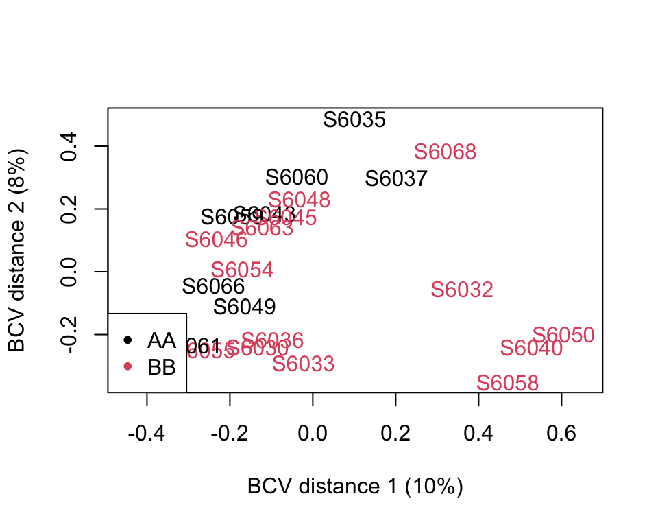
Figure 10.1: EdgeR (BVC distance)
## [1] "TaxaID" "Block" "Enrichment"
## [4] "Pvalue" "AdjustedPvalue" "logFC"
## [7] "logCPM" "LR" "Log2FoldChange (Median)\nAA_vs_BB"
## [10] "Median Abundance\n(All)" "Median Abundance\nAA" "Median Abundance\nBB"
## [13] "Log2FoldChange (Mean)\nAA_vs_BB" "Mean Abundance\n(All)" "Mean Abundance\nAA"
## [16] "Mean Abundance\nBB" "Occurrence (100%)\n(All)" "Occurrence (100%)\nAA"
## [19] "Occurrence (100%)\nBB" "Odds Ratio (95% CI)"## TaxaID Block Enrichment Pvalue AdjustedPvalue logFC logCPM LR Log2FoldChange (Median)\nAA_vs_BB
## 1 g__Acidaminococcus 9_AA vs 14_BB Nonsignif 0.006331806 0.06339772 -3.6537692 11.624194 7.4533622 NA
## 2 g__Actinomyces 9_AA vs 14_BB Nonsignif 0.068349670 0.19562147 1.8820292 11.004313 3.3222153 -0.9577718
## 3 g__Adlercreutzia 9_AA vs 14_BB Nonsignif 0.018855166 0.09205757 2.3817310 8.875209 5.5148986 NA
## 4 g__Agathobacter 9_AA vs 14_BB Nonsignif 0.299740178 0.51830072 -1.1273701 13.563968 1.0753498 0.1524904
## 5 g__Akkermansia 9_AA vs 14_BB Nonsignif 0.062219098 0.19562147 2.5474093 10.225497 3.4772223 NA
## 6 g__Alistipes 9_AA vs 14_BB Nonsignif 0.603600741 0.79522002 -0.4839035 11.355143 0.2695992 -0.1085245
## Median Abundance\n(All) Median Abundance\nAA Median Abundance\nBB Log2FoldChange (Mean)\nAA_vs_BB Mean Abundance\n(All)
## 1 0 0 0.0 1.7051442 58.82609
## 2 30 26 50.5 -1.3107676 50.91304
## 3 0 0 9.0 -2.4683647 19.21739
## 4 316 329 296.0 1.7488297 996.26087
## 5 0 0 0.0 -2.1676332 93.78261
## 6 64 64 69.0 0.2000385 163.86957
## Mean Abundance\nAA Mean Abundance\nBB Occurrence (100%)\n(All) Occurrence (100%)\nAA Occurrence (100%)\nBB Odds Ratio (95% CI)
## 1 101.777778 31.21429 21.74 22.22 21.43 0.67 (-0.11;1.5)
## 2 26.777778 66.42857 82.61 88.89 78.57 4.1 (6.8;1.3)
## 3 5.111111 28.28571 43.48 33.33 50.00 8.6 (13;4.3)
## 4 1740.444444 517.85714 65.22 55.56 71.43 0.39 (-1.4;2.2)
## 5 30.000000 134.78571 21.74 22.22 21.43 1.5 (2.3;0.71)
## 6 177.888889 154.85714 73.91 77.78 71.43 0.88 (0.64;1.1)Results:
The results comprises more than 10 columns, and the details as follow:
TaxaID: taxa name;
Block: groups’ names and numbers;
Enrichment: enriched direction based on Median Abundance and AdjustedPvalue;
logFC: fitted coefficient represents the fold-change for group AA and group BB;
logCPM: is the average expression of all samples for that particular gene across all samples on the log-scale expressed in counts per million (cpm, as calculated by edgeR after normalization);
LR: the signed likelihood ratio test statistic;
Pvalue and AdjustedPvalue: significant level of Pvalue and Adjusted-pvalue;
**Log2FoldChange (Median)_vs_BB**: Log2FoldChange (Median Abundance) between group AA and group BB;
Median Abundance (All)/(group AA)/(group BB): Median Abundance in all, group AA and group BB, respectively;
**Log2FoldChange (Mean)_vs_BB**: Log2FoldChange (Mean Abundance) between group AA and group BB;
Mean Abundance (All)/(group AA)/(group BB): Mean Abundance in all, group AA and group BB, respectively;
Occurrence (All)/(group AA)/(group BB): Occurrence in all, group AA and group BB, respectively;
Odds Ratio (95% CI): 95% confidence interval odds ratio between group AA and group BB.
other options for EdgeR
if (0) {
DA_edger <- run_edger(
data_otu = phyloseq::otu_table(dada2_ps_genus_filter_trim),
data_sam = phyloseq::sample_data(dada2_ps_genus_filter_trim),
group = "Group",
group_names = c("AA", "BB"))
DA_edger <- run_edger(
ps = dada2_ps,
taxa_level = "Genus",
group = "Group",
group_names = c("AA", "BB"))
DA_edger <- run_da(
ps = dada2_ps_genus_filter_trim,
group = "Group",
group_names = c("AA", "BB"),
da_method = "edger")
head(DA_edger)
}10.3.12 ANCOM
ANCOM (Analysis of composition of microbiomes) is from Analysis of composition of microbiomes: a novel method for studying microbial composition”, Microbial Ecology in Health (Mandal et al. 2015). ANCOM makes no distributional assumptions and can be implemented in a linear model framework. (Caution: the otu_table must be integers).
DA_ancom <- run_ancom(
ps = dada2_ps_genus_filter_trim,
group = "Group",
group_names = c("AA", "BB"))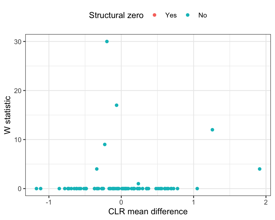
Figure 10.2: ANCOM (Structure Zero)
## [1] "TaxaID" "Block" "Enrichment"
## [4] "EffectSize" "(W)q-values < alpha" "W_ratio"
## [7] "detected_0.7" "Log2FoldChange (Median)\nAA_vs_BB" "Median Abundance\n(All)"
## [10] "Median Abundance\nAA" "Median Abundance\nBB" "Log2FoldChange (Mean)\nAA_vs_BB"
## [13] "Mean Abundance\n(All)" "Mean Abundance\nAA" "Mean Abundance\nBB"
## [16] "Occurrence (100%)\n(All)" "Occurrence (100%)\nAA" "Occurrence (100%)\nBB"
## [19] "Odds Ratio (95% CI)"## TaxaID Block Enrichment EffectSize (W)q-values < alpha W_ratio detected_0.7 Log2FoldChange (Median)\nAA_vs_BB
## 1 g__Acidaminococcus 9_AA vs 14_BB Nonsignif 0.05598359 0 0 FALSE NA
## 2 g__Actinomyces 9_AA vs 14_BB Nonsignif 0.77737041 0 0 FALSE -0.9577718
## 3 g__Adlercreutzia 9_AA vs 14_BB Nonsignif 0.24671418 0 0 FALSE NA
## 4 g__Agathobacter 9_AA vs 14_BB Nonsignif -0.51435011 0 0 FALSE 0.1524904
## 5 g__Akkermansia 9_AA vs 14_BB Nonsignif -0.07133173 0 0 FALSE NA
## 6 g__Alistipes 9_AA vs 14_BB Nonsignif 0.09952748 0 0 FALSE -0.1085245
## Median Abundance\n(All) Median Abundance\nAA Median Abundance\nBB Log2FoldChange (Mean)\nAA_vs_BB Mean Abundance\n(All)
## 1 0 0 0.0 1.7051442 58.82609
## 2 30 26 50.5 -1.3107676 50.91304
## 3 0 0 9.0 -2.4683647 19.21739
## 4 316 329 296.0 1.7488297 996.26087
## 5 0 0 0.0 -2.1676332 93.78261
## 6 64 64 69.0 0.2000385 163.86957
## Mean Abundance\nAA Mean Abundance\nBB Occurrence (100%)\n(All) Occurrence (100%)\nAA Occurrence (100%)\nBB Odds Ratio (95% CI)
## 1 101.777778 31.21429 21.74 22.22 21.43 0.67 (-0.11;1.5)
## 2 26.777778 66.42857 82.61 88.89 78.57 4.1 (6.8;1.3)
## 3 5.111111 28.28571 43.48 33.33 50.00 8.6 (13;4.3)
## 4 1740.444444 517.85714 65.22 55.56 71.43 0.39 (-1.4;2.2)
## 5 30.000000 134.78571 21.74 22.22 21.43 1.5 (2.3;0.71)
## 6 177.888889 154.85714 73.91 77.78 71.43 0.88 (0.64;1.1)Results:
The results comprises more than 10 columns, and the details as follow:
TaxaID: taxa name;
Block: groups’ names and numbers;
Enrichment: enriched direction based on Median Abundance and AdjustedPvalue;
EffectSize: effect size by ANCOM;
(W)q-values < alpha: q-values less than alpha;
W_ratio: the ratio of W values;
detected_0.7: W_ratio more than 0.7;
**Log2FoldChange (Median)_vs_BB**: Log2FoldChange (Median Abundance) between group AA and group BB;
Median Abundance (All)/(group AA)/(group BB): Median Abundance in all, group AA and group BB, respectively;
**Log2FoldChange (Mean)_vs_BB**: Log2FoldChange (Mean Abundance) between group AA and group BB;
Mean Abundance (All)/(group AA)/(group BB): Mean Abundance in all, group AA and group BB, respectively;
Occurrence (All)/(group AA)/(group BB): Occurrence in all, group AA and group BB, respectively;
Odds Ratio (95% CI): 95% confidence interval odds ratio between group AA and group BB.
other options for ANCOM
if (0) {
DA_ancom <- run_ancom(
data_otu = phyloseq::otu_table(dada2_ps_genus_filter_trim),
data_sam = phyloseq::sample_data(dada2_ps_genus_filter_trim),
group = "Group",
group_names = c("AA", "BB"))
DA_ancom <- run_ancom(
ps = dada2_ps,
taxa_level = "Genus",
group = "Group",
group_names = c("AA", "BB"))
DA_ancom <- run_da(
ps = dada2_ps_genus_filter_trim,
group = "Group",
group_names = c("AA", "BB"),
da_method = "ancom")
head(DA_ancom)
}10.3.13 Corncob
Corncob package is from Modeling microbial abundances and dysbiosis with beta-binomial regression”, Microbial Ecology in Health (Martin, Witten, and Willis 2020). Corncob is based on beta-binomial regression. (Caution: the otu_table must be integers).
if (0) {
DA_corncob <- run_corncob(
ps = dada2_ps_genus_filter_trim,
group = "Group",
group_names = c("AA", "BB"),
method = "Wald")
colnames(DA_ancom)
head(DA_ancom)
}other options for Corncob
if (0) {
DA_corncob <- run_corncob(
data_otu = phyloseq::otu_table(dada2_ps_genus_filter_trim),
data_sam = phyloseq::sample_data(dada2_ps_genus_filter_trim),
group = "Group",
group_names = c("AA", "BB"),
method = "Wald")
DA_corncob <- run_corncob(
ps = dada2_ps,
taxa_level = "Genus",
group = "Group",
group_names = c("AA", "BB"),
method = "Wald")
DA_corncob <- run_da(
ps = dada2_ps_genus_filter_trim,
group = "Group",
group_names = c("AA", "BB"),
da_method = "corncob",
method = "Wald")
head(DA_corncob)
}10.3.14 Maaslin2 (Microbiome Multivariable Association with Linear Models)
Maaslin2 package is from Multivariable association discovery in population-scale meta-omics studies (Mallick et al. 2021). Maaslin2 relies on general linear models to accommodate most modern epidemiological study designs, including cross-sectional and longitudinal, along with a variety of filtering, normalization, and transform methods.
if (0) {
DA_maaslin2 <- run_maaslin2(
ps = dada2_ps_genus_filter_trim,
group = "Group",
group_names = c("AA", "BB"),
transform = "LOG",
norm = "TMM",
method = "LM",
outdir = "./demo_output")
DA_maaslin2 <- run_maaslin2(
ps = dada2_ps,
taxa_level = "Genus",
group = "Group",
group_names = c("AA", "BB"),
transform = "LOG",
norm = "TMM",
method = "LM",
outdir = "./demo_output")
DA_maaslin2 <- run_maaslin2(
data_otu = phyloseq::otu_table(dada2_ps_genus_filter_trim),
data_sam = phyloseq::sample_data(dada2_ps_genus_filter_trim),
group = "Group",
group_names = c("AA", "BB"),
transform = "LOG",
norm = "TMM",
method = "LM",
outdir = "./demo_output")
DA_maaslin2 <- run_da(
ps = dada2_ps_genus_filter_trim,
group = "Group",
group_names = c("AA", "BB"),
da_method = "maaslin2",
transform = "LOG",
norm = "TMM",
method = "LM",
outdir = "./demo_output")
head(DA_maaslin2)
}10.3.15 LOCOM
LOCOM: A logistic regression model for testing differential abundance in compositional microbiome data with false discovery rate control (Hu, Satten, and Hu 2022).
Cautions: It reports an error information which the matrix is singularError when user uses low prev.cut.
library(permute)
DA_locom <- run_locom(ps = dada2_ps_genus_filter_trim,
group = "Group",
group_names = c("AA", "BB"),
fdr.nominal = 0.2,
prev.cut = 0.8)## Warning: glm.fit: fitted probabilities numerically 0 or 1 occurred
## Warning: glm.fit: fitted probabilities numerically 0 or 1 occurred
## Warning: glm.fit: fitted probabilities numerically 0 or 1 occurred## 71 OTU(s) with fewer than 18.4 in all samples are removed
## permutations: 1## TaxaID Block EffectSize Pvalue AdjustedPvalue Log2FoldChange (Median)\nAA_vs_BB Median Abundance\n(All)
## 1 g__Bacteroides 9_AA vs 14_BB 1.030 0.024 0.12 1.5367266 3807
## 2 g__Blautia 9_AA vs 14_BB 0.570 0.034 0.12 0.2641697 8199
## 3 g__Lachnoclostridium 9_AA vs 14_BB 0.672 0.040 0.12 0.7874146 422
## 4 g__Lactobacillus 9_AA vs 14_BB -3.180 0.028 0.12 -3.0334230 56
## Median Abundance\nAA Median Abundance\nBB Log2FoldChange (Mean)\nAA_vs_BB Mean Abundance\n(All) Mean Abundance\nAA Mean Abundance\nBB
## 1 9103 3137.5 0.9841180 5745.5652 8219.44444 4155.2143
## 2 8645 7198.5 0.3178904 9145.9565 10397.55556 8341.3571
## 3 485 281.0 0.4658394 417.9565 502.33333 363.7143
## 4 24 196.5 -5.0905713 791.2609 37.44444 1275.8571
## Occurrence (100%)\n(All) Occurrence (100%)\nAA Occurrence (100%)\nBB Odds Ratio (95% CI)
## 1 100.00 100.00 100.00 0.45 (-1.1;2)
## 2 100.00 100.00 100.00 0.62 (-0.3;1.5)
## 3 95.65 100.00 92.86 0.63 (-0.27;1.5)
## 4 86.96 77.78 92.86 1.8e+08 (1.8e+08;1.8e+08)Results:
The results comprises more than 10 columns, and the details as follow:
TaxaID: taxa name;
Block: groups’ names and numbers;
EffectSize: effect size by ANCOM;
Pvalue: p-values for OTU-specific tests;
AdjustedPvalue : q-values (adjusted p-values by the BH procedure) for OTU-specific tests;
**Log2FoldChange (Median)_vs_BB**: Log2FoldChange (Median Abundance) between group AA and group BB;
Median Abundance (All)/(group AA)/(group BB): Median Abundance in all, group AA and group BB, respectively;
**Log2FoldChange (Mean)_vs_BB**: Log2FoldChange (Mean Abundance) between group AA and group BB;
Mean Abundance (All)/(group AA)/(group BB): Mean Abundance in all, group AA and group BB, respectively;
Occurrence (All)/(group AA)/(group BB): Occurrence in all, group AA and group BB, respectively;
Odds Ratio (95% CI): 95% confidence interval odds ratio between group AA and group BB.
10.4 Metagenomic sequencing microbial data (metaphlan2/3)
10.4.1 Wilcoxon Rank Sum and Signed Rank Tests
Wilcoxon Rank Sum and Signed Rank Tests, which are nonparameter test methods, use the rank of taxa abundance to find the significant taxa.
DA_wilcox_mgs <- run_wilcox(
ps = metaphlan2_ps_genus_filter_trim,
group = "Group",
group_names = c("AA", "BB"))
colnames(DA_wilcox_mgs)## [1] "TaxaID" "Block" "Enrichment"
## [4] "EffectSize" "Statistic" "Pvalue"
## [7] "AdjustedPvalue" "Log2FoldChange (Median)\nAA_vs_BB" "Median Abundance\n(All)"
## [10] "Median Abundance\nAA" "Median Abundance\nBB" "Log2FoldChange (Rank)\nAA_vs_BB"
## [13] "Mean Rank Abundance\nAA" "Mean Rank Abundance\nBB" "Occurrence (100%)\n(All)"
## [16] "Occurrence (100%)\nAA" "Occurrence (100%)\nBB" "Odds Ratio (95% CI)"## TaxaID Block Enrichment EffectSize Statistic Pvalue AdjustedPvalue Log2FoldChange (Median)\nAA_vs_BB
## 1 g__Acidaminococcus 7_AA vs 15_BB Nonsignif 0.9966151 36.0 0.19074499 0.52578545 NA
## 2 g__Adlercreutzia 7_AA vs 15_BB Nonsignif 0.5416258 28.0 0.05769072 0.20413638 NA
## 3 g__Alistipes 7_AA vs 15_BB Nonsignif 1.6269577 71.0 0.20193465 0.52578545 2.061604
## 4 g__Anaerostipes 7_AA vs 15_BB Nonsignif 0.3278059 31.0 0.13834560 0.42425985 -4.964322
## 5 g__Anaerotruncus 7_AA vs 15_BB Nonsignif 0.8349750 47.5 0.71288708 0.81982014 NA
## 6 g__Bacteroides 7_AA vs 15_BB Nonsignif 0.9956964 85.0 0.02128483 0.09495645 1.229057
## Median Abundance\n(All) Median Abundance\nAA Median Abundance\nBB Log2FoldChange (Rank)\nAA_vs_BB Mean Rank Abundance\nAA
## 1 0.00000000 0.0000000 0.0000000 -0.4631577 9.14
## 2 0.00000000 0.0000000 0.0000558 -0.7147950 8.00
## 3 0.00711780 0.0236665 0.0056693 0.4613459 14.14
## 4 0.00031435 0.0000229 0.0007149 -0.6171177 8.43
## 5 0.00000000 0.0000000 0.0000000 -0.1327552 10.79
## 6 0.24894650 0.4568864 0.1949060 0.7906916 16.14
## Mean Rank Abundance\nBB Occurrence (100%)\n(All) Occurrence (100%)\nAA Occurrence (100%)\nBB Odds Ratio (95% CI)
## 1 12.60 36.36 14.29 46.67 8700 (8700;8700)
## 2 13.13 40.91 14.29 53.33 Inf (Inf;Inf)
## 3 10.27 77.27 71.43 80.00 0.22 (-2.7;3.2)
## 4 12.93 86.36 71.43 93.33 6 (9.5;2.5)
## 5 11.83 36.36 28.57 40.00 1.3 (1.8;0.78)
## 6 9.33 100.00 100.00 100.00 0.31 (-2;2.6)10.4.2 Liner discriminant analysis (LDA) effect size (LEfSe)
LEfSe method is from Metagenomic biomarker discovery and explanation (Segata et al. 2011). It uses Liner discriminant analysis model to identify Differential Taxa.
# DA_lefse_mgs <- run_lefse(
# ps = metaphlan2_ps_genus_filter_trim,
# group = "Group",
# group_names = c("AA", "BB"),
# norm = "CPM",
# Lda = 2)
DA_lefse_mgs <- run_lefse2(
ps = metaphlan2_ps_genus_filter_trim,
group = "Group",
group_names = c("AA", "BB"),
norm = "CPM",
lda_cutoff = 2)
colnames(DA_lefse_mgs)## [1] "TaxaID" "Block" "LDA_Score"
## [4] "Enrichment" "EffectSize" "Pvalue"
## [7] "Log2FoldChange (Median)\nAA_vs_BB" "Median Abundance\n(All)" "Median Abundance\nAA"
## [10] "Median Abundance\nBB" "Log2FoldChange (Mean)\nAA_vs_BB" "Mean Abundance\n(All)"
## [13] "Mean Abundance\nAA" "Mean Abundance\nBB" "Occurrence (100%)\n(All)"
## [16] "Occurrence (100%)\nAA" "Occurrence (100%)\nBB" "Odds Ratio (95% CI)"## TaxaID Block LDA_Score Enrichment EffectSize Pvalue Log2FoldChange (Median)\nAA_vs_BB Median Abundance\n(All)
## 1 g__Bacteroides 7_AA vs 15_BB -5.379223 AA 2.5356524 0.021966365 1.190538 254267.6272
## 2 g__Bifidobacterium 7_AA vs 15_BB 5.170414 BB 2.8199931 0.003440517 -6.574737 39083.6006
## 3 g__Blautia 7_AA vs 15_BB 4.496247 BB 0.5696647 0.001046123 -3.203712 21823.6865
## 4 g__Collinsella 7_AA vs 15_BB 4.229420 BB 2.4346418 0.019909355 NA 7739.0203
## 5 g__Dorea 7_AA vs 15_BB 4.208815 BB 2.0503963 0.004294461 -5.725635 8556.6787
## 6 g__Eggerthella 7_AA vs 15_BB 3.659350 BB 1.2390028 0.047014415 NA 591.5818
## Median Abundance\nAA Median Abundance\nBB Log2FoldChange (Mean)\nAA_vs_BB Mean Abundance\n(All) Mean Abundance\nAA Mean Abundance\nBB
## 1 464614.8499 203566.1197 1.141008 291728.672 465019.4054 210859.663
## 2 917.9094 87496.9227 -3.459750 114237.628 14608.6929 160731.132
## 3 3704.9909 34135.0398 -2.335372 25770.580 6855.3562 34597.684
## 4 0.0000 11644.4661 -2.928408 12502.243 2269.5616 17277.494
## 5 270.5248 14315.1145 -3.454703 11345.173 1455.6962 15960.262
## 6 0.0000 771.5754 -3.764261 2232.472 232.9684 3165.574
## Occurrence (100%)\n(All) Occurrence (100%)\nAA Occurrence (100%)\nBB Odds Ratio (95% CI)
## 1 100.00 100.00 100.00 0.32 (-1.9;2.5)
## 2 100.00 100.00 100.00 150 (160;140)
## 3 100.00 100.00 100.00 92 (100;83)
## 4 68.18 42.86 80.00 20 (25;14)
## 5 90.91 71.43 100.00 28 (34;21)
## 6 63.64 42.86 73.33 430 (450;420)10.4.3 t-test
T test, a parametric test method, identifies the significant taxa.
DA_ttest_mgs <- run_ttest(
ps = metaphlan2_ps_genus_filter_trim,
group = "Group",
group_names = c("AA", "BB"))
colnames(DA_ttest_mgs)## [1] "TaxaID" "Block" "Enrichment"
## [4] "EffectSize" "Statistic" "Pvalue"
## [7] "AdjustedPvalue" "Log2FoldChange (Median)\nAA_vs_BB" "Median Abundance\n(All)"
## [10] "Median Abundance\nAA" "Median Abundance\nBB" "Log2FoldChange (Mean)\nAA_vs_BB"
## [13] "Mean Abundance\n(All)" "Mean Abundance\nAA" "Mean Abundance\nBB"
## [16] "Occurrence (100%)\n(All)" "Occurrence (100%)\nAA" "Occurrence (100%)\nBB"
## [19] "Odds Ratio (95% CI)"## TaxaID Block Enrichment EffectSize Statistic Pvalue AdjustedPvalue Log2FoldChange (Median)\nAA_vs_BB
## 1 g__Acidaminococcus 7_AA vs 15_BB Nonsignif 0.9966151 -1.0515590 0.31074638 0.6151313 NA
## 2 g__Adlercreutzia 7_AA vs 15_BB Nonsignif 0.5416258 -2.1929042 0.04570343 0.2102358 NA
## 3 g__Alistipes 7_AA vs 15_BB Nonsignif 1.6269577 1.5963681 0.15951558 0.5119489 2.061604
## 4 g__Anaerostipes 7_AA vs 15_BB Nonsignif 0.3278059 -1.6970563 0.10937430 0.4192682 -4.964322
## 5 g__Anaerotruncus 7_AA vs 15_BB Nonsignif 0.8349750 -0.5871152 0.56369794 0.6823712 NA
## 6 g__Bacteroides 7_AA vs 15_BB Nonsignif 0.9956964 2.2882319 0.04545820 0.2102358 1.229057
## Median Abundance\n(All) Median Abundance\nAA Median Abundance\nBB Log2FoldChange (Mean)\nAA_vs_BB Mean Abundance\n(All)
## 1 0.00000000 0.0000000 0.0000000 -4.6280567 0.0095489955
## 2 0.00000000 0.0000000 0.0000558 -9.2633214 0.0008266409
## 3 0.00711780 0.0236665 0.0056693 2.1761109 0.0199576000
## 4 0.00031435 0.0000229 0.0007149 -2.2827694 0.0016651773
## 5 0.00000000 0.0000000 0.0000000 -0.9025366 0.0002137000
## 6 0.24894650 0.4568864 0.1949060 1.1807675 0.2848799364
## Mean Abundance\nAA Mean Abundance\nBB Occurrence (100%)\n(All) Occurrence (100%)\nAA Occurrence (100%)\nBB Odds Ratio (95% CI)
## 1 5.558857e-04 0.0137457800 36.36 14.29 46.67 8700 (8700;8700)
## 2 1.971429e-06 0.0012114867 40.91 14.29 53.33 Inf (Inf;Inf)
## 3 4.254910e-02 0.0094149000 77.27 71.43 80.00 0.22 (-2.7;3.2)
## 4 4.579714e-04 0.0022285400 86.36 71.43 93.33 6 (9.5;2.5)
## 5 1.341714e-04 0.0002508133 36.36 28.57 40.00 1.3 (1.8;0.78)
## 6 4.602683e-01 0.2030320467 100.00 100.00 100.00 0.31 (-2;2.6)10.4.4 Maaslin2 (Microbiome Multivariable Association with Linear Models)
Maaslin2 package is from Multivariable association discovery in population-scale meta-omics studies (Mallick et al. 2021). Maaslin2 relies on general linear models to accommodate most modern epidemiological study designs, including cross-sectional and longitudinal, along with a variety of filtering, normalization, and transform methods.
10.5 Visualization
The Volcano plot is used to display differential analysis. plot_volcano provides multiple parameters for plotting volcano. More details to see help(plot_volcano).
The barplot is used to display the lefse results.
10.5.1 Volcano plot
The X and Y coordinate axis are flexible to choose for Volcano. Here, we choose logFC and AdjustedPvalue to visualize the results
DA_limma_voom <- run_limma_voom(
ps = dada2_ps_genus_filter_trim,
group = "Group",
group_names = c("AA", "BB"))
colnames(DA_limma_voom)## [1] "TaxaID" "Block" "Enrichment"
## [4] "EffectSize" "logFC" "Pvalue"
## [7] "AdjustedPvalue" "Log2FoldChange (Median)\nAA_vs_BB" "Median Abundance\n(All)"
## [10] "Median Abundance\nAA" "Median Abundance\nBB" "Log2FoldChange (Mean)\nAA_vs_BB"
## [13] "Mean Abundance\n(All)" "Mean Abundance\nAA" "Mean Abundance\nBB"
## [16] "Occurrence (100%)\n(All)" "Occurrence (100%)\nAA" "Occurrence (100%)\nBB"
## [19] "Odds Ratio (95% CI)"DA_limma_voom_volcano <- plot_volcano(
da_res = DA_limma_voom,
group_names = c("AA", "BB"),
x_index = "logFC",
x_index_cutoff = 0.5,
y_index = "Pvalue",
y_index_cutoff = 0.05,
group_color = c("red", "grey", "blue"),
topN = 5)
DA_limma_voom_volcano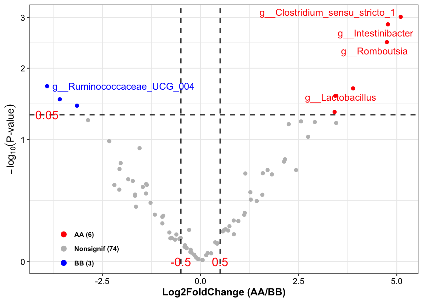
Figure 10.3: Volcano (limma-voom: logFC and AdjustedPvalue)
plot_volcano(
da_res = DA_limma_voom,
group_names = c("AA", "BB"),
x_index = "logFC",
x_index_cutoff = 0.5,
y_index = "Pvalue",
y_index_cutoff = 0.05,
group_color = c("red", "grey", "blue"),
topN = 5,
add_enrich_arrow = TRUE)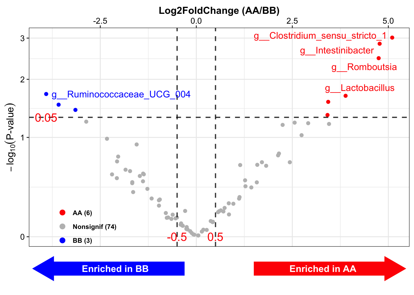
Figure 10.4: Volcano with arrow (limma-voom: logFC and AdjustedPvalue)
DA_limma_voom_volcano effectsize
plot_volcano(
da_res = DA_limma_voom,
group_names = c("AA", "BB"),
x_index = "EffectSize",
x_index_cutoff = 1,
y_index = "Pvalue",
y_index_cutoff = 0.05,
group_color = c("red", "grey", "blue"),
topN = 8)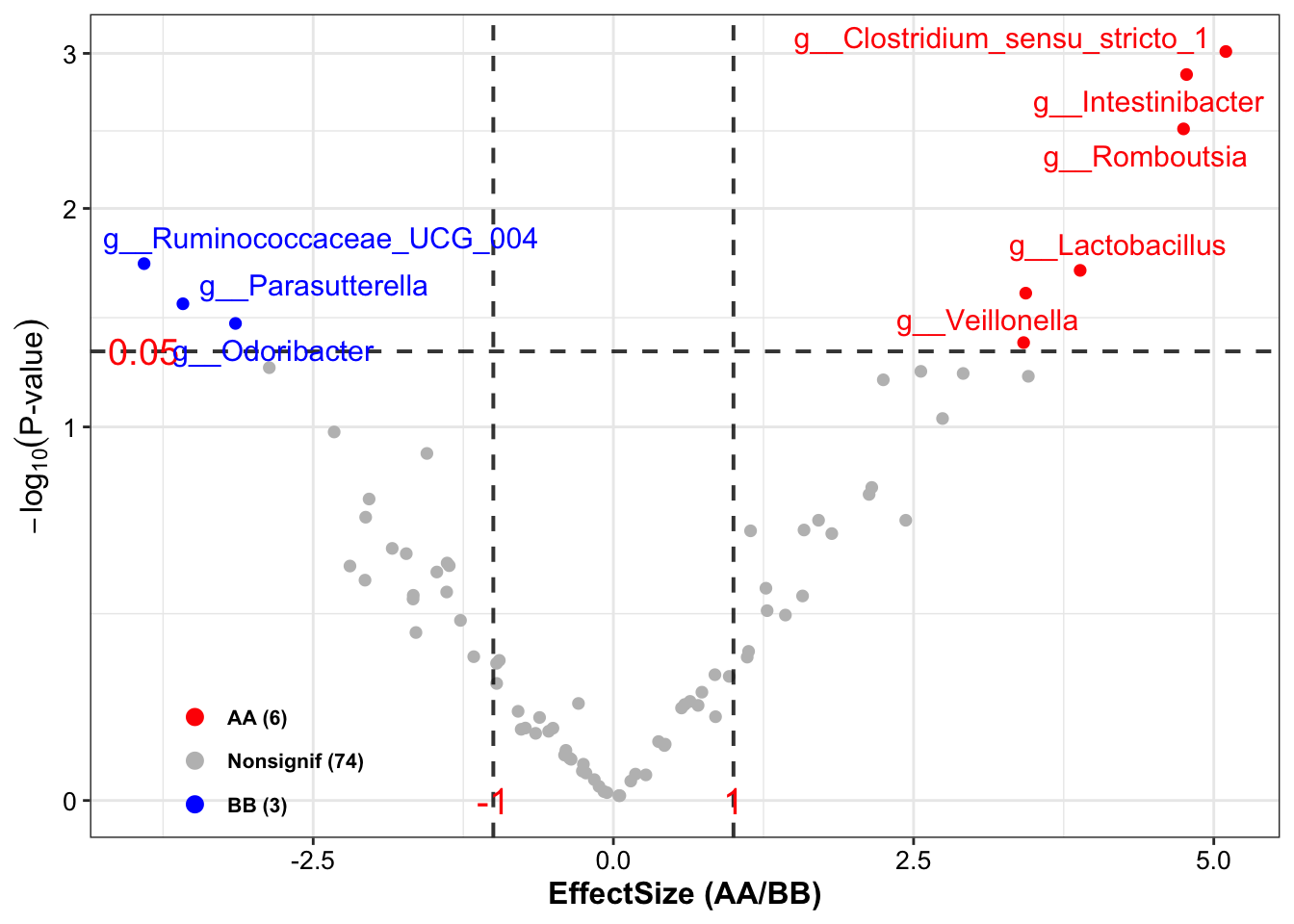
Figure 10.5: Volcano (limma-voom: EffectSize and Pvalue)
The logFC and EffectSize are the same values in limma-voom.
10.5.2 barplot in lefse
# DA_lefse <- run_lefse(
# ps = dada2_ps_genus_filter_trim,
# group = "Group",
# group_names = c("AA", "BB"),
# norm = "CPM",
# Lda = 2)
DA_lefse <- run_lefse2(
ps = dada2_ps_genus_filter_trim,
group = "Group",
group_names = c("AA", "BB"),
norm = "CPM",
lda_cutoff = 2)
# # don't run this code when you do lefse in reality
# DA_lefse$LDA_Score <- DA_lefse$LDA_Score * 1000
plot_lefse(
da_res = DA_lefse,
x_index = "LDA_Score",
x_index_cutoff = 1,
group_color = c("green", "red")) 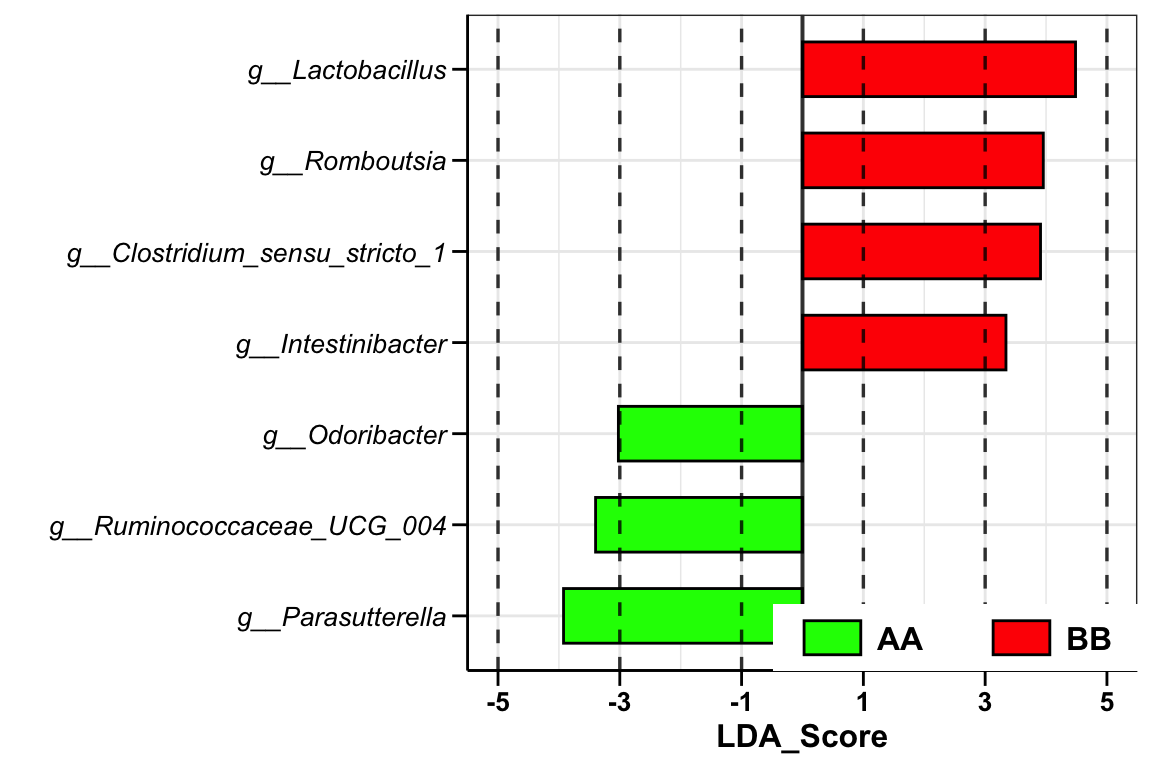
Figure 10.6: Barplot (Lefse)
10.6 Dominant taxa
Display the significant taxa with selection using boxplot.
DA_wilcox <- run_wilcox(
ps = metaphlan2_ps_genus_filter_trim,
group = "Group",
group_names = c("AA", "BB"))
plot_topN_boxplot(
ps = metaphlan2_ps_genus_filter_trim,
da_res = DA_wilcox,
x_index = "Log2FoldChange (Median)\nAA_vs_BB",
x_index_cutoff = 0.2,
y_index = "Pvalue",
y_index_cutoff = 0.3,
topN = 3,
taxa_name = "s__Ruminococcus_torques",
group = "Group")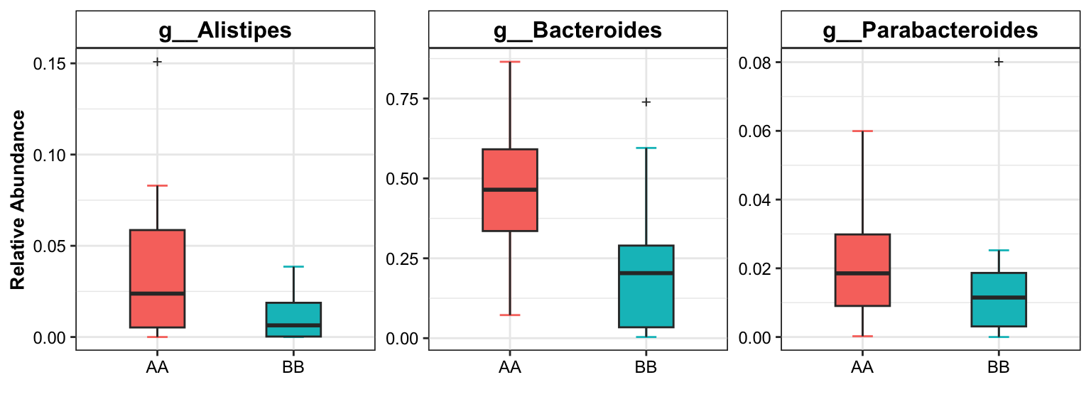
Figure 10.7: Dominant Taxa
10.7 Multiple differential analysis by one function
here, we provide the run_multiple_da for obtaining the results list from multiple differential analysis methods.
multiple_res <- run_multiple_da(
ps = dada2_ps_genus_filter_trim,
group = "Group",
group_names = c("AA", "BB"),
da_method = c("aldex", "limma_voom", "mbzinb", "omnibus"),
p_adjust = "none")## |------------(25%)----------(50%)----------(75%)----------|
## Start GMPR normalization ...
## Start Winsorization ...
## Perform filtering ...
## --A total of  82  taxa will be tested with a sample size of 23 !
## --Omnibus test is selected!
## --Dispersion is treated as a parameter of interest!
## Start testing ...
## 10 %
## 20 %
## 30 %
## 40 %
## 50 %
## 60 %
## 70 %
## 80 %
## 90 %
## 100%!
## Handle failed taxa using permutation test!
## Permutation test ....
## Completed!## [1] "aldex" "limma_voom" "mbzinb" "omnibus"- plot results
plot_multiple_DA(
    Multip_DA_res = multiple_res,
    x_index_list = c("EffectSize", "logFC", "mean.LFC", "abund.LFC.CompvarBB.est"),
    x_index_cutoff = 0,
    y_index = "AdjustedPvalue",
    y_index_cutoff = 0.5,
    cellwidth = 50,
    cellheight = 10)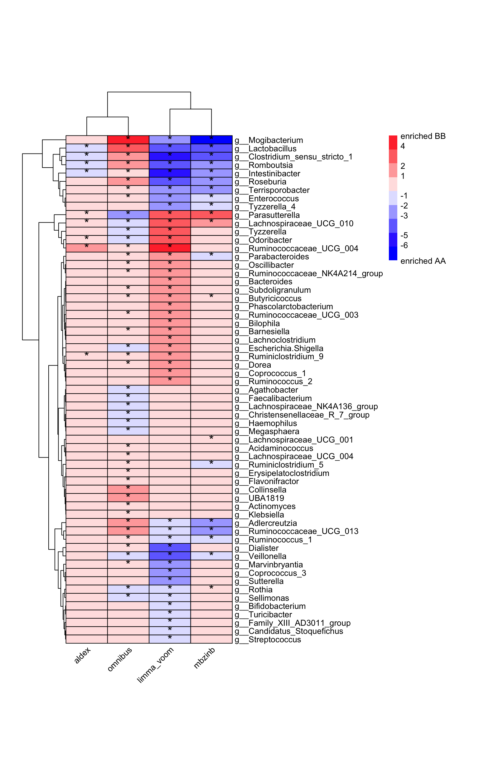
Figure 10.8: Multiple DA results
10.8 Systematic Information
## ─ Session info ───────────────────────────────────────────────────────────────────────────────────────────────────────────────────────────
##  setting  value
##  version  R version 4.1.3 (2022-03-10)
##  os       macOS Monterey 12.2.1
##  system   x86_64, darwin17.0
##  ui       RStudio
##  language (EN)
##  collate  en_US.UTF-8
##  ctype    en_US.UTF-8
##  tz       Asia/Shanghai
##  date     2023-11-30
##  rstudio  2023.09.0+463 Desert Sunflower (desktop)
##  pandoc   3.1.1 @ /Applications/RStudio.app/Contents/Resources/app/quarto/bin/tools/ (via rmarkdown)
##
## ─ Packages ───────────────────────────────────────────────────────────────────────────────────────────────────────────────────────────────
##  package              * version   date (UTC) lib source
##  abind                  1.4-5     2016-07-21 [2] CRAN (R 4.1.0)
##  ade4                   1.7-22    2023-02-06 [2] CRAN (R 4.1.2)
##  ALDEx2                 1.30.0    2022-11-01 [2] Bioconductor
##  annotate               1.72.0    2021-10-26 [2] Bioconductor
##  AnnotationDbi          1.60.2    2023-03-10 [2] Bioconductor
##  ape                  * 5.7-1     2023-03-13 [2] CRAN (R 4.1.2)
##  askpass                1.1       2019-01-13 [2] CRAN (R 4.1.0)
##  backports              1.4.1     2021-12-13 [2] CRAN (R 4.1.0)
##  base64enc              0.1-3     2015-07-28 [2] CRAN (R 4.1.0)
##  bayesm                 3.1-5     2022-12-02 [2] CRAN (R 4.1.2)
##  Biobase                2.54.0    2021-10-26 [2] Bioconductor
##  BiocGenerics           0.40.0    2021-10-26 [2] Bioconductor
##  BiocParallel           1.28.3    2021-12-09 [2] Bioconductor
##  biomformat             1.22.0    2021-10-26 [2] Bioconductor
##  Biostrings             2.62.0    2021-10-26 [2] Bioconductor
##  bit                    4.0.5     2022-11-15 [2] CRAN (R 4.1.2)
##  bit64                  4.0.5     2020-08-30 [2] CRAN (R 4.1.0)
##  bitops                 1.0-7     2021-04-24 [2] CRAN (R 4.1.0)
##  blob                   1.2.4     2023-03-17 [2] CRAN (R 4.1.2)
##  bookdown               0.34      2023-05-09 [2] CRAN (R 4.1.2)
##  broom                  1.0.5     2023-06-09 [2] CRAN (R 4.1.3)
##  bslib                  0.6.0     2023-11-21 [1] CRAN (R 4.1.3)
##  cachem                 1.0.8     2023-05-01 [2] CRAN (R 4.1.2)
##  callr                  3.7.3     2022-11-02 [2] CRAN (R 4.1.2)
##  car                    3.1-2     2023-03-30 [2] CRAN (R 4.1.2)
##  carData                3.0-5     2022-01-06 [2] CRAN (R 4.1.2)
##  caTools                1.18.2    2021-03-28 [2] CRAN (R 4.1.0)
##  checkmate              2.2.0     2023-04-27 [2] CRAN (R 4.1.2)
##  cli                    3.6.1     2023-03-23 [2] CRAN (R 4.1.2)
##  cluster                2.1.4     2022-08-22 [2] CRAN (R 4.1.2)
##  coda                   0.19-4    2020-09-30 [2] CRAN (R 4.1.0)
##  codetools              0.2-19    2023-02-01 [2] CRAN (R 4.1.2)
##  coin                   1.4-2     2021-10-08 [2] CRAN (R 4.1.0)
##  colorspace             2.1-0     2023-01-23 [2] CRAN (R 4.1.2)
##  compositions           2.0-6     2023-04-13 [2] CRAN (R 4.1.2)
##  conflicted           * 1.2.0     2023-02-01 [2] CRAN (R 4.1.2)
##  corrplot               0.92      2021-11-18 [2] CRAN (R 4.1.0)
##  cowplot                1.1.1     2020-12-30 [2] CRAN (R 4.1.0)
##  crayon                 1.5.2     2022-09-29 [2] CRAN (R 4.1.2)
##  crosstalk              1.2.0     2021-11-04 [2] CRAN (R 4.1.0)
##  data.table             1.14.8    2023-02-17 [2] CRAN (R 4.1.2)
##  DBI                    1.1.3     2022-06-18 [2] CRAN (R 4.1.2)
##  DelayedArray           0.20.0    2021-10-26 [2] Bioconductor
##  DEoptimR               1.0-14    2023-06-09 [2] CRAN (R 4.1.3)
##  DESeq2                 1.34.0    2021-10-26 [2] Bioconductor
##  devtools               2.4.5     2022-10-11 [2] CRAN (R 4.1.2)
##  digest                 0.6.33    2023-07-07 [1] CRAN (R 4.1.3)
##  dplyr                * 1.1.2     2023-04-20 [2] CRAN (R 4.1.2)
##  DT                     0.28      2023-05-18 [2] CRAN (R 4.1.3)
##  edgeR                  3.36.0    2021-10-26 [2] Bioconductor
##  ellipsis               0.3.2     2021-04-29 [2] CRAN (R 4.1.0)
##  emmeans                1.8.7     2023-06-23 [1] CRAN (R 4.1.3)
##  estimability           1.4.1     2022-08-05 [2] CRAN (R 4.1.2)
##  evaluate               0.21      2023-05-05 [2] CRAN (R 4.1.2)
##  FactoMineR             2.8       2023-03-27 [2] CRAN (R 4.1.2)
##  fansi                  1.0.4     2023-01-22 [2] CRAN (R 4.1.2)
##  farver                 2.1.1     2022-07-06 [2] CRAN (R 4.1.2)
##  fastmap                1.1.1     2023-02-24 [2] CRAN (R 4.1.2)
##  flashClust             1.01-2    2012-08-21 [2] CRAN (R 4.1.0)
##  foreach                1.5.2     2022-02-02 [2] CRAN (R 4.1.2)
##  foreign                0.8-84    2022-12-06 [2] CRAN (R 4.1.2)
##  Formula                1.2-5     2023-02-24 [2] CRAN (R 4.1.2)
##  fs                     1.6.2     2023-04-25 [2] CRAN (R 4.1.2)
##  genefilter             1.76.0    2021-10-26 [2] Bioconductor
##  geneplotter            1.72.0    2021-10-26 [2] Bioconductor
##  generics               0.1.3     2022-07-05 [2] CRAN (R 4.1.2)
##  GenomeInfoDb           1.30.1    2022-01-30 [2] Bioconductor
##  GenomeInfoDbData       1.2.7     2022-03-09 [2] Bioconductor
##  GenomicRanges          1.46.1    2021-11-18 [2] Bioconductor
##  ggiraph                0.8.7     2023-03-17 [2] CRAN (R 4.1.2)
##  ggiraphExtra           0.3.0     2020-10-06 [2] CRAN (R 4.1.2)
##  ggplot2              * 3.4.2     2023-04-03 [2] CRAN (R 4.1.2)
##  ggpubr               * 0.6.0     2023-02-10 [2] CRAN (R 4.1.2)
##  ggrepel                0.9.3     2023-02-03 [2] CRAN (R 4.1.2)
##  ggsci                  3.0.0     2023-03-08 [2] CRAN (R 4.1.2)
##  ggsignif               0.6.4     2022-10-13 [2] CRAN (R 4.1.2)
##  glmnet                 4.1-7     2023-03-23 [2] CRAN (R 4.1.2)
##  glue                   1.6.2     2022-02-24 [2] CRAN (R 4.1.2)
##  gplots                 3.1.3     2022-04-25 [2] CRAN (R 4.1.2)
##  gridExtra              2.3       2017-09-09 [2] CRAN (R 4.1.0)
##  gtable                 0.3.3     2023-03-21 [2] CRAN (R 4.1.2)
##  gtools                 3.9.4     2022-11-27 [2] CRAN (R 4.1.2)
##  highr                  0.10      2022-12-22 [2] CRAN (R 4.1.2)
##  Hmisc                  5.1-0     2023-05-08 [2] CRAN (R 4.1.2)
##  htmlTable              2.4.1     2022-07-07 [2] CRAN (R 4.1.2)
##  htmltools              0.5.7     2023-11-03 [1] CRAN (R 4.1.3)
##  htmlwidgets            1.6.2     2023-03-17 [2] CRAN (R 4.1.2)
##  httpuv                 1.6.11    2023-05-11 [2] CRAN (R 4.1.3)
##  httr                   1.4.6     2023-05-08 [2] CRAN (R 4.1.2)
##  igraph                 1.5.0     2023-06-16 [1] CRAN (R 4.1.3)
##  insight                0.19.3    2023-06-29 [2] CRAN (R 4.1.3)
##  IRanges                2.28.0    2021-10-26 [2] Bioconductor
##  iterators              1.0.14    2022-02-05 [2] CRAN (R 4.1.2)
##  jquerylib              0.1.4     2021-04-26 [2] CRAN (R 4.1.0)
##  jsonlite               1.8.7     2023-06-29 [2] CRAN (R 4.1.3)
##  kableExtra             1.3.4     2021-02-20 [2] CRAN (R 4.1.2)
##  KEGGREST               1.34.0    2021-10-26 [2] Bioconductor
##  KernSmooth             2.23-22   2023-07-10 [2] CRAN (R 4.1.3)
##  knitr                  1.43      2023-05-25 [2] CRAN (R 4.1.3)
##  labeling               0.4.2     2020-10-20 [2] CRAN (R 4.1.0)
##  later                  1.3.1     2023-05-02 [2] CRAN (R 4.1.2)
##  lattice              * 0.21-8    2023-04-05 [2] CRAN (R 4.1.2)
##  leaps                  3.1       2020-01-16 [2] CRAN (R 4.1.0)
##  libcoin                1.0-9     2021-09-27 [2] CRAN (R 4.1.0)
##  lifecycle              1.0.3     2022-10-07 [2] CRAN (R 4.1.2)
##  limma                  3.50.3    2022-04-07 [2] Bioconductor
##  locfit                 1.5-9.8   2023-06-11 [2] CRAN (R 4.1.3)
##  LOCOM                  1.1       2022-08-05 [2] Github (yijuanhu/LOCOM@c181e0f)
##  magrittr               2.0.3     2022-03-30 [2] CRAN (R 4.1.2)
##  MASS                   7.3-60    2023-05-04 [2] CRAN (R 4.1.2)
##  Matrix                 1.6-0     2023-07-08 [2] CRAN (R 4.1.3)
##  MatrixGenerics         1.6.0     2021-10-26 [2] Bioconductor
##  matrixStats            1.0.0     2023-06-02 [2] CRAN (R 4.1.3)
##  mbzinb                 0.2       2022-03-16 [2] local
##  memoise                2.0.1     2021-11-26 [2] CRAN (R 4.1.0)
##  metagenomeSeq          1.36.0    2021-10-26 [2] Bioconductor
##  mgcv                   1.8-42    2023-03-02 [2] CRAN (R 4.1.2)
##  microbiome             1.16.0    2021-10-26 [2] Bioconductor
##  mime                   0.12      2021-09-28 [2] CRAN (R 4.1.0)
##  miniUI                 0.1.1.1   2018-05-18 [2] CRAN (R 4.1.0)
##  modeltools             0.2-23    2020-03-05 [2] CRAN (R 4.1.0)
##  multcomp               1.4-25    2023-06-20 [2] CRAN (R 4.1.3)
##  multcompView           0.1-9     2023-04-09 [2] CRAN (R 4.1.2)
##  multtest               2.50.0    2021-10-26 [2] Bioconductor
##  munsell                0.5.0     2018-06-12 [2] CRAN (R 4.1.0)
##  mvtnorm                1.2-2     2023-06-08 [2] CRAN (R 4.1.3)
##  mycor                  0.1.1     2018-04-10 [2] CRAN (R 4.1.0)
##  NADA                   1.6-1.1   2020-03-22 [2] CRAN (R 4.1.0)
##  nlme                 * 3.1-162   2023-01-31 [2] CRAN (R 4.1.2)
##  nnet                   7.3-19    2023-05-03 [2] CRAN (R 4.1.2)
##  openssl                2.0.6     2023-03-09 [2] CRAN (R 4.1.2)
##  permute              * 0.9-7     2022-01-27 [2] CRAN (R 4.1.2)
##  pheatmap               1.0.12    2019-01-04 [2] CRAN (R 4.1.0)
##  phyloseq             * 1.38.0    2021-10-26 [2] Bioconductor
##  picante              * 1.8.2     2020-06-10 [2] CRAN (R 4.1.0)
##  pillar                 1.9.0     2023-03-22 [2] CRAN (R 4.1.2)
##  pkgbuild               1.4.2     2023-06-26 [2] CRAN (R 4.1.3)
##  pkgconfig              2.0.3     2019-09-22 [2] CRAN (R 4.1.0)
##  pkgload                1.3.2.1   2023-07-08 [2] CRAN (R 4.1.3)
##  plyr                   1.8.8     2022-11-11 [2] CRAN (R 4.1.2)
##  png                    0.1-8     2022-11-29 [2] CRAN (R 4.1.2)
##  ppcor                  1.1       2015-12-03 [2] CRAN (R 4.1.0)
##  prettyunits            1.1.1     2020-01-24 [2] CRAN (R 4.1.0)
##  processx               3.8.2     2023-06-30 [2] CRAN (R 4.1.3)
##  profvis                0.3.8     2023-05-02 [2] CRAN (R 4.1.2)
##  promises               1.2.0.1   2021-02-11 [2] CRAN (R 4.1.0)
##  protoclust             1.6.4     2022-04-01 [2] CRAN (R 4.1.2)
##  ps                     1.7.5     2023-04-18 [2] CRAN (R 4.1.2)
##  pscl                   1.5.5.1   2023-05-10 [2] CRAN (R 4.1.2)
##  purrr                  1.0.1     2023-01-10 [2] CRAN (R 4.1.2)
##  qvalue                 2.26.0    2021-10-26 [2] Bioconductor
##  R6                     2.5.1     2021-08-19 [2] CRAN (R 4.1.0)
##  RAIDA                  1.0       2022-03-14 [2] local
##  RColorBrewer         * 1.1-3     2022-04-03 [2] CRAN (R 4.1.2)
##  Rcpp                   1.0.11    2023-07-06 [1] CRAN (R 4.1.3)
##  RcppZiggurat           0.1.6     2020-10-20 [2] CRAN (R 4.1.0)
##  RCurl                  1.98-1.12 2023-03-27 [2] CRAN (R 4.1.2)
##  remotes                2.4.2     2021-11-30 [2] CRAN (R 4.1.0)
##  reshape2               1.4.4     2020-04-09 [2] CRAN (R 4.1.0)
##  reticulate             1.30      2023-06-09 [2] CRAN (R 4.1.3)
##  Rfast                  2.0.8     2023-07-03 [2] CRAN (R 4.1.3)
##  rhdf5                  2.38.1    2022-03-10 [2] Bioconductor
##  rhdf5filters           1.6.0     2021-10-26 [2] Bioconductor
##  Rhdf5lib               1.16.0    2021-10-26 [2] Bioconductor
##  rlang                  1.1.1     2023-04-28 [1] CRAN (R 4.1.2)
##  rmarkdown              2.23      2023-07-01 [2] CRAN (R 4.1.3)
##  robustbase             0.99-0    2023-06-16 [2] CRAN (R 4.1.3)
##  rpart                  4.1.19    2022-10-21 [2] CRAN (R 4.1.2)
##  RSpectra               0.16-1    2022-04-24 [2] CRAN (R 4.1.2)
##  RSQLite                2.3.1     2023-04-03 [2] CRAN (R 4.1.2)
##  rstatix                0.7.2     2023-02-01 [2] CRAN (R 4.1.2)
##  rstudioapi             0.15.0    2023-07-07 [2] CRAN (R 4.1.3)
##  Rtsne                  0.16      2022-04-17 [2] CRAN (R 4.1.2)
##  rvest                  1.0.3     2022-08-19 [2] CRAN (R 4.1.2)
##  S4Vectors              0.32.4    2022-03-29 [2] Bioconductor
##  sandwich               3.0-2     2022-06-15 [2] CRAN (R 4.1.2)
##  sass                   0.4.6     2023-05-03 [2] CRAN (R 4.1.2)
##  scales                 1.2.1     2022-08-20 [2] CRAN (R 4.1.2)
##  scatterplot3d          0.3-44    2023-05-05 [2] CRAN (R 4.1.2)
##  sessioninfo            1.2.2     2021-12-06 [2] CRAN (R 4.1.0)
##  shape                  1.4.6     2021-05-19 [2] CRAN (R 4.1.0)
##  shiny                  1.7.4.1   2023-07-06 [2] CRAN (R 4.1.3)
##  sjlabelled             1.2.0     2022-04-10 [2] CRAN (R 4.1.2)
##  sjmisc                 2.8.9     2021-12-03 [2] CRAN (R 4.1.0)
##  stringi                1.7.12    2023-01-11 [2] CRAN (R 4.1.2)
##  stringr                1.5.0     2022-12-02 [2] CRAN (R 4.1.2)
##  SummarizedExperiment   1.24.0    2021-10-26 [2] Bioconductor
##  survival               3.5-5     2023-03-12 [2] CRAN (R 4.1.2)
##  svglite                2.1.1     2023-01-10 [2] CRAN (R 4.1.2)
##  systemfonts            1.0.4     2022-02-11 [2] CRAN (R 4.1.2)
##  tensorA                0.36.2    2020-11-19 [2] CRAN (R 4.1.0)
##  TH.data                1.1-2     2023-04-17 [2] CRAN (R 4.1.2)
##  tibble               * 3.2.1     2023-03-20 [2] CRAN (R 4.1.2)
##  tidyr                  1.3.0     2023-01-24 [2] CRAN (R 4.1.2)
##  tidyselect             1.2.0     2022-10-10 [2] CRAN (R 4.1.2)
##  truncnorm              1.0-9     2023-03-20 [2] CRAN (R 4.1.2)
##  umap                   0.2.10.0  2023-02-01 [2] CRAN (R 4.1.2)
##  urlchecker             1.0.1     2021-11-30 [2] CRAN (R 4.1.0)
##  usethis                2.2.2     2023-07-06 [2] CRAN (R 4.1.3)
##  utf8                   1.2.3     2023-01-31 [2] CRAN (R 4.1.2)
##  uuid                   1.1-0     2022-04-19 [2] CRAN (R 4.1.2)
##  vctrs                  0.6.3     2023-06-14 [1] CRAN (R 4.1.3)
##  vegan                * 2.6-4     2022-10-11 [2] CRAN (R 4.1.2)
##  viridis              * 0.6.3     2023-05-03 [2] CRAN (R 4.1.2)
##  viridisLite          * 0.4.2     2023-05-02 [2] CRAN (R 4.1.2)
##  webshot                0.5.5     2023-06-26 [2] CRAN (R 4.1.3)
##  withr                  2.5.0     2022-03-03 [2] CRAN (R 4.1.2)
##  Wrench                 1.12.0    2021-10-26 [2] Bioconductor
##  xfun                   0.40      2023-08-09 [1] CRAN (R 4.1.3)
##  XMAS2                * 2.2.0     2023-11-30 [1] local
##  XML                    3.99-0.14 2023-03-19 [2] CRAN (R 4.1.2)
##  xml2                   1.3.5     2023-07-06 [2] CRAN (R 4.1.3)
##  xtable                 1.8-4     2019-04-21 [2] CRAN (R 4.1.0)
##  XVector                0.34.0    2021-10-26 [2] Bioconductor
##  yaml                   2.3.7     2023-01-23 [2] CRAN (R 4.1.2)
##  zCompositions          1.4.0-1   2022-03-26 [2] CRAN (R 4.1.2)
##  zlibbioc               1.40.0    2021-10-26 [2] Bioconductor
##  zoo                    1.8-12    2023-04-13 [2] CRAN (R 4.1.2)
##
##  [1] /Users/zouhua/Library/R/x86_64/4.1/library
##  [2] /Library/Frameworks/R.framework/Versions/4.1/Resources/library
##
## ──────────────────────────────────────────────────────────────────────────────────────────────────────────────────────────────────────────