Chapter 7 Beta diversity
Beta diversity: Measures for differences between samples from different groups to identify if there are differences in the overall community composition and structure.
Here, we not only Check the homogeneity condition, but also perform Permutational Multivariate Analysis of Variance (PERMANOVA) and Ordination including PCA, PCoA and UMAP to explore the significance on microbiota data.
Outline of this Chapter:
7.2 Importing Data
data("dada2_ps")
dada2_ps_remove_BRS <- get_GroupPhyloseq(
                         ps = dada2_ps,
                         group = "Group",
                         group_names = "QC",
                         discard = TRUE)
dada2_ps_rarefy <- norm_rarefy(object = dada2_ps_remove_BRS,
                               size = 51181)
dada2_ps_rarefy
## phyloseq-class experiment-level object
## otu_table() OTU Table: [ 891 taxa and 23 samples ]
## sample_data() Sample Data: [ 23 samples by 1 sample variables ]
## tax_table() Taxonomy Table: [ 891 taxa by 7 taxonomic ranks ]
## phy_tree() Phylogenetic Tree: [ 891 tips and 888 internal nodes ]
## refseq() DNAStringSet: [ 891 reference sequences ]MGS dataset
data("metaphlan2_ps")
metaphlan2_ps_remove_BRS <- get_GroupPhyloseq(
                               ps = metaphlan2_ps,
                               group = "Group",
                               group_names = "QC",
                               discard = TRUE)
metaphlan2_ps_remove_BRS
## phyloseq-class experiment-level object
## otu_table() OTU Table: [ 326 taxa and 22 samples ]
## sample_data() Sample Data: [ 22 samples by 2 sample variables ]
## tax_table() Taxonomy Table: [ 326 taxa by 7 taxonomic ranks ]7.3 Phylogenetic beta-diversity metrics
7.3.1 Unweighted Unifrac
Unweighted Unifrac is based on presence/absence of different taxa and abundance is not important.
The UniFrac distance, also known as unweighted UniFrac distance, was introduced by Lozupone et al. The goal of the UniFrac distance metric was to enable objective comparison between microbiome samples from different conditions.
\[d^{u} = \sum^{n}_{i=1}\frac{b_{i}|I(p_{i}^{A} > 0) - I(p_{i}^{B} > 0)|}{\sum_{i=1}^{n}b_{i}}\]
where,
\(d^{u}\) = unweighted UniFrac distance;
\(A\), \(B\) = microbiome community A and B, respectively;
\(n\) = rooted phylogenetic tree’s branches;
\(b_{i}\) =length of the branch \(i\);
\(p_{i}^{A}\) and \(p_{i}^{A}\) = taxa proportions descending from the branch \(i\) for community A and B, respectively.
Calculation
- Visualization
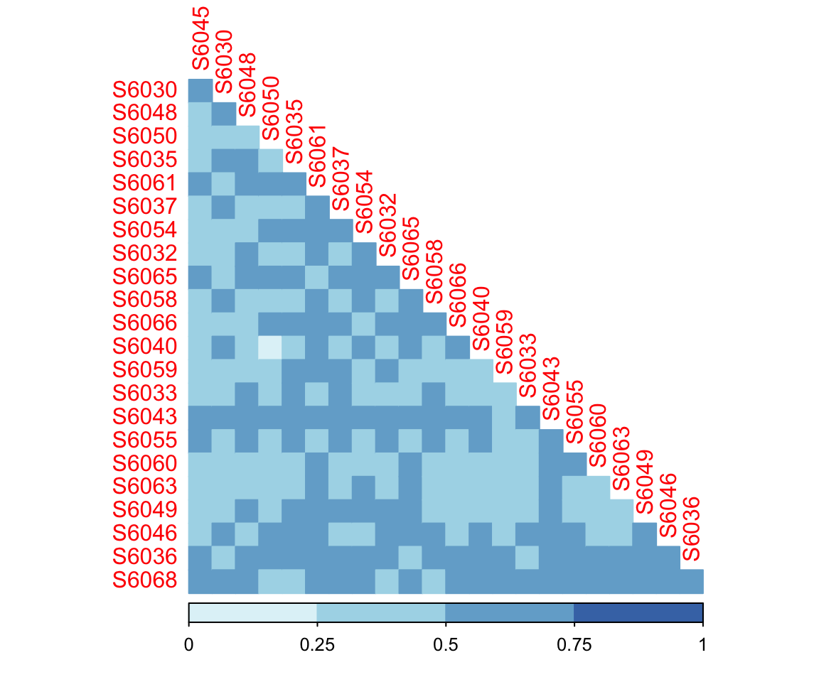
Figure 7.1: Unweighted Unifrac Distance
Try repeating the above ordination using filtered phyloseq object (discarding singletons/OTUs with very low reads).
7.3.2 Weighted Unifrac
Weighted Unifrac will consider the abundances of different taxa.
In 2007, Lozupone et al. added a proportional weighting to the original unweighted method, hence called this new UniFrac measure as weighted UniFrac.
The weighted UniFrac distance is defined as:
\[d^{W} = \frac{\sum_{i=1}^{n}b_{i}|p_{i}^{A}-p_{i}^{B}|}{\sum_{i=1}^{n}b_{i}(p_{i}^{A}+p_{i}^{B})}\]
where,
\(d^{W}\) = (normalized) weighted UniFrac distance;
\(A\), \(B\) = microbiome community A and B, respectively;
\(n\) = rooted phylogenetic tree’s branches;
\(b_{i}\) = length of the branch \(i\).
By adding a proportional weighting to UniFrac distance, weighted UniFrac distance reduces the problem of low abundance taxa being represented as a 0 or by a low count depending on sampling depth.
- Calculation
The result of dispersion test (Pr(>F) > 0.05) showed that the homogeneity condition of two groups were not significant.
- Visualization
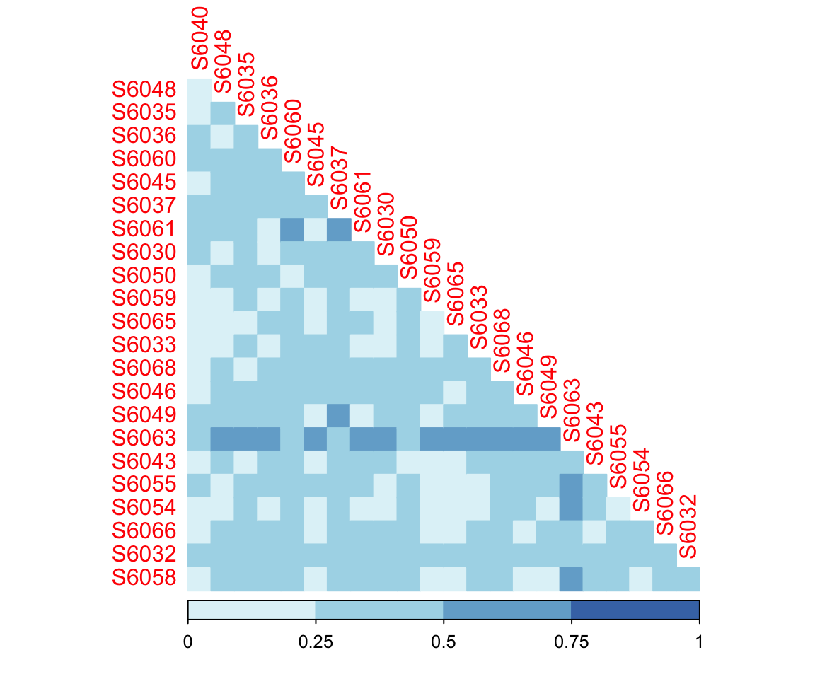
Figure 7.2: Weighted Unifrac Distance
7.3.3 Generalized UniFrac Distance Metrics
However, either unweighted or weighted UniFrac distances may not be very powerful in detecting change in moderately abundant lineages (J. Chen et al. 2012) because they assign too much weight either to rare lineages or to most abundant lineages. Thus, Chen et al. proposed the following generalized UniFrac distances to unify weighted UniFrac and unweighted UniFrac distances.
The Generalized UniFrac Distance Metrics is defined as:
\[d^{\alpha} = \frac{\sum_{i=1}^{n}b_{i}(p_{i}^{A}+p_{i}^{B})^{\alpha}|\frac{p_{i}^{A}-p_{i}^{B}}{p_{i}^{A}+p_{i}^{B}}|}{\sum_{i=1}^{n}b_{i}(p_{i}^{A}+p_{i}^{B})}\]
where,
\(d^{\alpha}\) = generalized UniFrac distances;
\(\alpha\in [0, 1]\) is used to controls the contribution from high-abundance branches;
Calculation
# approach1
dada2_beta <- run_beta_diversity(ps = dada2_ps_rarefy,
                                 method = "GUniFrac",
                                 GUniFrac_alpha = 0.5)

# approach2
dada2_otu_tab <- phyloseq::otu_table(dada2_ps_rarefy)
dada2_tree <- phyloseq::phy_tree(dada2_ps_rarefy)

dada2_unifracs <- run_GUniFrac(otu.tab = dada2_otu_tab,
                               tree = dada2_tree,
                               alpha = c(0, 0.5, 1))$unifracs

dada2_dw <- dada2_unifracs[, , "d_1"]    # Weighted UniFrac
dada2_du <- dada2_unifracs[, , "d_UW"]   # Unweighted UniFrac
dada2_dv <- dada2_unifracs[, , "d_VAW"]  # Variance adjusted weighted UniFrac
dada2_d0 <- dada2_unifracs[, , "d_0"]    # GUniFrac with alpha 0
dada2_d5 <- dada2_unifracs[, , "d_0.5"] # GUniFrac with alpha 0.5- Visualization: GUniFrac with alpha 0.5
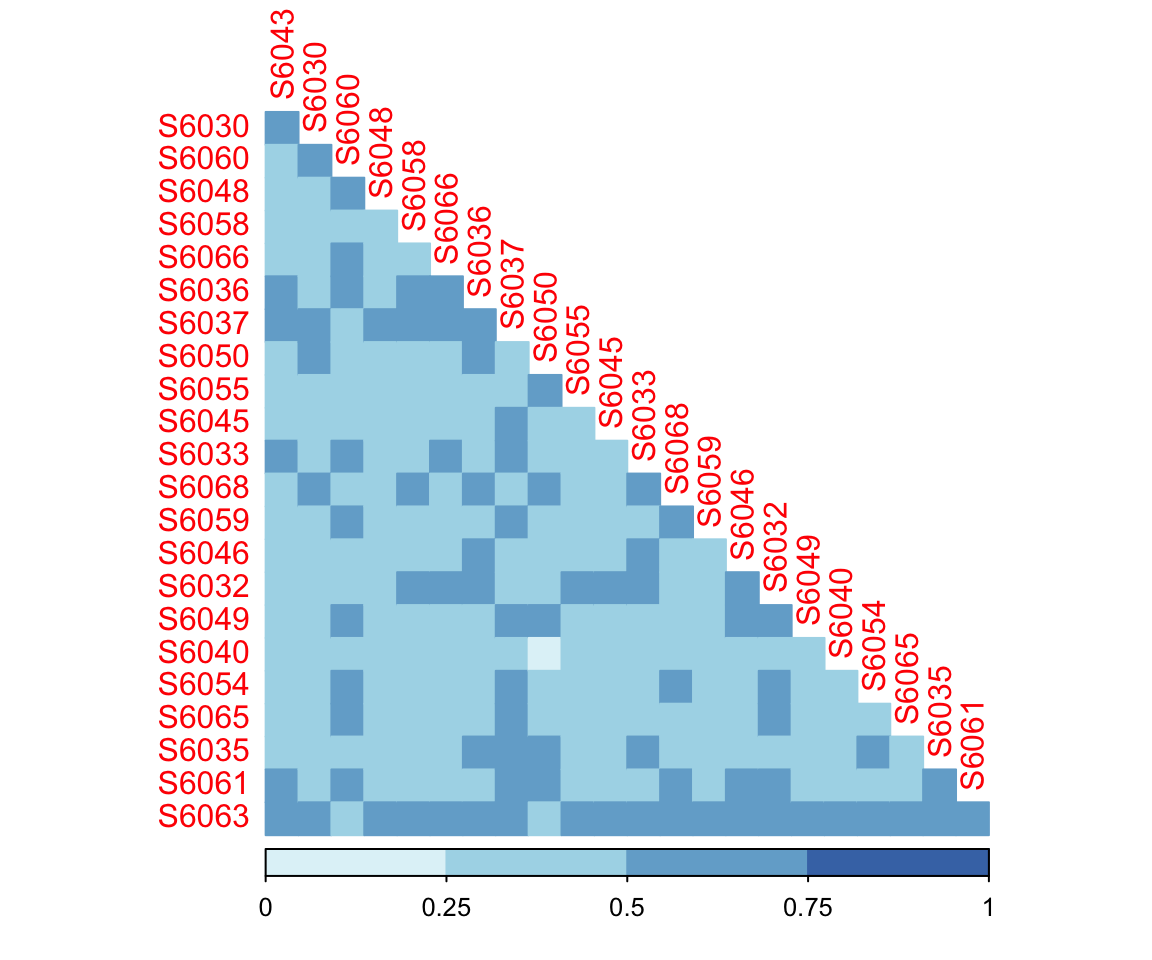
Figure 7.3: Generalized UniFrac Distance (alpha=0.5)
7.4 Distance (Dissimilarity) Coefficients: Bray-Curtis Index
For microbiome abundance data, the measures of distance coefficients are not really distances. They actually measure “dissimilarity”.
Measures of dissimilarity include Euclidian distance, Manhattan, and Bray-Curtis measures. Here, we take Bray-Curtis distance as an example.
As defined by Bray and Curtis, the index of dissimilarity is given as follow:
\[BC = \frac{\sum_{i=1}^{n}|X_{ij}-X_{ik}|}{\sum_{i=1}^{n}|X_{ij}+X_{ik}|}\] where,
\(BC\) Bray-Curtis measure of dissimilarity;
\(X_{ij}\), \(X_{ik}\) Number of individuals in species;
\(i\) in each \(sample (j, k)\);
\(n\) Total number of species in samples.
dada2_beta <- run_beta_diversity(ps = dada2_ps_rarefy,
                                 method = "bray")
plot_distance_corrplot(datMatrix = dada2_beta$BetaDistance)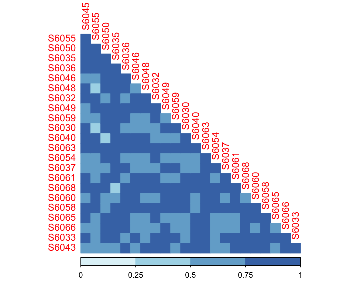
Figure 7.4: Bray Curtis Distance
7.5 Checking the homogeneity condition
- beta disdispersion
# dada2_beta <- run_beta_diversity(ps = dada2_ps_rarefy,
#                                  method = "jsd",
#                                  group = "Group")

run_beta_dispersion(ps = dada2_ps_rarefy,
                    method = "jsd",
                    group = "Group")
##
## Permutation test for homogeneity of multivariate dispersions
## Permutation: free
## Number of permutations: 999
##
## Response: Distances
## Df Sum Sq Mean Sq F N.Perm Pr(>F)
## Groups 1 0.000486 0.0004856 0.1207 999 0.725
## Residuals 21 0.084520 0.0040247
##
## Pairwise comparisons:
## (Observed p-value below diagonal, permuted p-value above diagonal)
## AA BB
## AA 0.735
## BB 0.73178## Df Sum Sq Mean Sq F N.Perm Pr(>F)
## Groups 1 0.0004856016 0.0004856016 0.1206542 999 0.725The result of dispersion test (Pr(>F) < 0.05) showed that the homogeneity condition of two groups were significant.
7.6 Permutational Multivariate Analysis of Variance (PERMANOVA)
Permutational Multivariate Analysis of Variance (PERMANOVA) test (Anderson 2014) is to investigate the associations between the environmental factors including discrete or continuous variables (treatments or populations representatives, age, gender etc) and the whole microbial community.
##       SumsOfSample Df SumsOfSqs   MeanSqs  F.Model         R2 Pr(>F) AdjustedPvalue
## Group 23 1 0.3126266 0.3126266 1.004313 0.04564163 0.444 0.444## SumsOfSample Df SumsOfSqs MeanSqs F.Model R2 Pr(>F) AdjustedPvalue
## TempRowNames 34 33 14.3104868 0.4336511 0.000000 1.00000000 1.000 1.0000000
## SampleType 34 3 4.6452206 1.5484069 4.806097 0.32460256 0.001 0.0090000
## Year 34 1 0.5943614 0.5943614 1.386657 0.04153327 0.120 0.3352500
## Month 34 4 1.5688911 0.3922228 0.892703 0.10963227 0.734 0.9437143
## Day 34 3 1.2450953 0.4150318 0.952972 0.08700579 0.561 0.9437143
## Subject 34 1 0.5816949 0.5816949 1.355854 0.04064816 0.149 0.3352500
## ReportedAntibioticUsage 34 1 0.5943614 0.5943614 1.386657 0.04153327 0.120 0.3352500
## DaysSinceExperimentStart 34 4 1.5688911 0.3922228 0.892703 0.10963227 0.734 0.9437143
## Description 34 33 14.3104868 0.4336511 0.000000 1.00000000 1.000 1.0000000Results:
The PERMANOVA result of the SampleType (AdjustedPvalue < 0.05) revealed that different groups of SampleType had the distinct patterns of microbial community. From the previous metadata, SampleType had four groups (gut, right palm, left palm, tongue) which are different body sites.
The other continuous variables such as Year, Day and Month didn’t show any significant association with microbial community.
We suggest you performing the PERMANOVA test before you do correlation analysis between individual taxa and environmental factors. If the whole microbial community had related to one environmental factor, we could find more associations between individual taxa and environmental factors.
Ordination analysis is usually utilized for dimensionality reduction and then we decipher their results by using scatterplot. In fact, we should combine the statistical results, for example PERMANOVA, ANOSIM or others and dimension reduction results to provide stronger evidences to display the association and difference.
7.7 Mantel Test
Mantel tests (Mantel 1967) are correlation tests that determine the correlation between two matrices (rather than two variables). When using the test for microbial ecology, the matrices are often distance/dissimilarity matrices with corresponding positions (i.e. samples in the same order in both matrices).
A significant Mantel test will tell you that the distances between samples in one matrix are correlated with the distances between samples in the other matrix. Therefore, as the distance between samples increases with respect to one matrix, the distances between the same samples also increases in the other matrix.
There are also three distance matrix for mantel test:
- Species abundance dissimilarity matrix: created using a distance measure, i.e. Bray-curtis dissimilarity. This is the same type of dissimilarity matrix used when conducting an ANOSIM test or when making an NMDS plot;
- Environmental factors distance matrix: generally created using Euclidean Distance;
- Geographic distance matrix: the physical distance between sites for z_distance (i.e. Haversine distance).
data("amplicon_ps")
run_MantelTest(
        ps = amplicon_ps,
        y_variables = c("SampleType", "Subject", "ReportedAntibioticUsage",
                        "DaysSinceExperimentStart", "Description"),
        z_variables = c("Year", "Month", "Day"),
        method_mantel = "mantel.partial",
        method_cor = "spearman",
        method_dist = c("bray", "euclidean", "jaccard"))
##
## Partial Mantel statistic based on Spearman's rank correlation rho
##
## Call:
## vegan::mantel.partial(xdis = x_dis, ydis = y_dis, zdis = z_dis, method = method_cor, permutations = 999)
##
## Mantel statistic r: 0.2897
## Significance: 0.001
##
## Upper quantiles of permutations (null model):
## 90% 95% 97.5% 99%
## 0.0531 0.0744 0.0901 0.1163
## Permutation: free
## Number of permutations: 999Results:
From the results, we could see that the y_dis (environmental factors) has a strong relationship with the OTU Bray-Curtis dissimiliarity matrix (Mantel statistic R: 0.3318, p value = 0.001) after adjusting the z_dis matrix. In other words, as samples become more dissimilar in terms of environmental factors, they also become more dissimilar in terms of microbial community composition.
Options for Mantel test
run_MantelTest(
        ps = amplicon_ps,
        y_variables = c("SampleType", "Subject", "ReportedAntibioticUsage",
                        "DaysSinceExperimentStart", "Description"),
        method_mantel = "mantel",
        method_cor = "spearman",
        method_dist = c("bray", "euclidean"))
##
## Mantel statistic based on Spearman's rank correlation rho
##
## Call:
## vegan::mantel(xdis = x_dis, ydis = y_dis, method = method_cor, permutations = 999)
##
## Mantel statistic r: 0.2661
## Significance: 0.001
##
## Upper quantiles of permutations (null model):
## 90% 95% 97.5% 99%
## 0.0619 0.0859 0.1081 0.1304
## Permutation: free
## Number of permutations: 999run_MantelTest(
ps = amplicon_ps,
y_variables = c("SampleType", "Subject", "ReportedAntibioticUsage",
"DaysSinceExperimentStart", "Description"),
method_mantel = "mantel.randtest",
method_cor = "spearman",
method_dist = c("bray", "euclidean"))## Monte-Carlo test
## Call: ade4::mantel.randtest(m1 = x_dis, m2 = y_dis, nrepet = 999)
##
## Observation: 0.2819519
##
## Based on 999 replicates
## Simulated p-value: 0.001
## Alternative hypothesis: greater
##
## Std.Obs Expectation Variance
## 7.1085392424 0.0004079774 0.00156867037.8 Analysis of Similarity (ANOSIM)
Analysis of Similarity (ANOSIM) is simply a modified version of the Mantel Test based on a standardized rank correlation between two distance matrices.
It is a nonparametric procedure for testing the hypothesis of no difference between two or more groups of samples based on permutation test of among-and within-group similarities.
The ANOSIM test statistic(R) is based on the difference of mean ranks between groups and within groups. It is given below:
\[R = \frac{\bar{r}_{B} - \bar{r}_{W}}{M/2}\] where,
\(R\) test statistic, is an index of relative within-group dissimilarity;
\(M = N(N − 1)/2\) number of sample pairs;
\(N\) is the total number of samples (subjects);
\(r_{B}\) is the mean of the ranked similarity between groups;
\(r_{W}\) is the mean of the ranked similarity within groups.
##
## Call:
## vegan::anosim(x = dis, grouping = datphe, permutations = 999)
## Dissimilarity: bray
##
## ANOSIM statistic R: -0.03337
##       Significance: 0.63
##
## Permutation: free
## Number of permutations: 999
The p-value of 0.62 is more than 0.05, which indicates that within-group similarity is not greater or less than between-group similarity at 0.05 significant level. We can conclude that there is no strong evidence that the within-group samples are more different than would be expected by random chance.
7.9 Multi-response permutation procedures (MRPP)
Multi-response permutation procedures (MRPP) (Mielke Jr 1991) is a nonparametric procedure for testing the hypothesis of no difference between two or more groups of samples based on permutation test of among-and within-group dissimilarities.
##
## Call:
## vegan::mrpp(dat = dis, grouping = datphe, permutations = 999)
##
## Dissimilarity index: bray
## Weights for groups:  n
##
## Class means and counts:
##
##       AA     BB
## delta 0.7736 0.785
## n     9      14
##
## Chance corrected within-group agreement A: 0.0006646
## Based on observed delta 0.7805 and expected delta 0.781
##
## Significance of delta: 0.428
## Permutation: free
## Number of permutations: 999
The observed and expected deltas are 0.6469 and 0.851, respectively. The significance of delta is 0.001 with the chance corrected within-group agreement A of 0.2399. We conclude that there is statistically significant difference of the four SampleType at the 0.05 of significance level.
7.10 Ordination
Ordination is one of the main multivariate methods to reduce the dimensions of taxa–for instance, the whole microbial community often contains too much taxa which makes the microbial profile have too large dimensions. Utilizing ordination to convert the data into two or three dimensions could have more interpretable visualization. Compared to clustering methods, ordination focuses on the dimension reduction and has explanation loss (variation).
We also use a distance method to calculate the distance matrix among samples and then do ordination analysis. Here, we give five universal ordination methods. There is no one-fit-all method for all microbiota data, so please pay attention to your own ordination analysis.
7.10.1 Principal Component Analysis (PCA)
Principal Component Analysis (PCA) uses a linear combination algorithm to obtain the principal components (PC) (the number of PCs according to the samples). The results have been effected by the normalization methods because different count numbers would affect the PCs. We recommend you using filtering or normalization before performing PCA.
7.10.1.1 Preprocessing phyloseq object
data("dada2_ps")

# step1: Removing samples of specific group in phyloseq-class object
dada2_ps_remove_BRS <- get_GroupPhyloseq(
                     ps = dada2_ps,
                     group = "Group",
                     group_names = "QC")

# step2: Rarefying counts in phyloseq-class object
dada2_ps_rarefy <- norm_rarefy(object = dada2_ps_remove_BRS,
                               size = 51181)

# step3: Extracting specific taxa phyloseq-class object
dada2_ps_rare_genus <- summarize_taxa(ps = dada2_ps_rarefy,
                                      taxa_level = "Genus",
                                      absolute = TRUE)

# step4: Aggregating low relative abundance or unclassified taxa into others
# dada2_ps_genus_LRA <- summarize_LowAbundance_taxa(ps = dada2_ps_rare_genus,
#                                                   cutoff = 10,
#                                                   unclass = TRUE)

# step4: Filtering the low relative abundance or unclassified taxa by the threshold
dada2_ps_genus_filter <- run_filter(ps = dada2_ps_rare_genus,
                                    cutoff = 10,
                                    unclass = TRUE)

# step5: Trimming the taxa with low occurrence less than threshold
dada2_ps_genus_filter_trim <- run_trim(object = dada2_ps_genus_filter,
                                       cutoff = 0.2,
                                       trim = "feature")
dada2_ps_genus_filter_trim
## phyloseq-class experiment-level object
## otu_table() OTU Table: [ 83 taxa and 23 samples ]
## sample_data() Sample Data: [ 23 samples by 1 sample variables ]
## tax_table() Taxonomy Table: [ 83 taxa by 6 taxonomic ranks ]7.10.1.2 Running PCA
ordination_PCA <- run_ordination(
                       ps = dada2_ps_genus_filter_trim,
                       group = "Group",
                       method = "PCA")

names(ordination_PCA)
## [1] "fit" "dat" "explains" "eigvalue" "PERMANOVA" "BETADISPER" "axis_taxa_cor"The object of run_ordination is comprising of several results which could be used for visualization.
fit: the result of PCA functions from
stats::prcomp;dat: the combination of PCs score and metadata group information;
explains: the 1st and 2nd PCs’ explains;
eigvalue: the eigvalues of all the PCs;
PERMANOVA: the result of PERMANOVA between the whole microbial community and group;
axis_taxa_cor: inherit from the
XVIZpackage for visualization (only for PCoA analysis).
7.10.1.3 Visualization
plot_Ordination provides too many parameters for users to display the ordination results by using ggplot2 format. Here is the ordinary pattern.
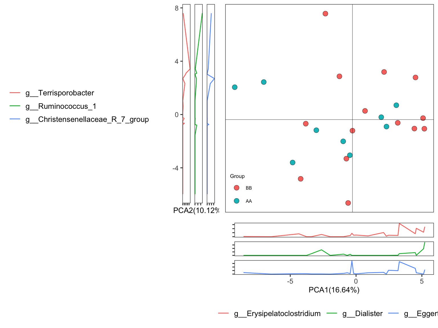
Figure 7.5: Principal Component Analysis (PCA): Ordinary pattern
Results:
Scatterplot showed the distribution of samples in the two groups;
PERMANOVA results revealed that there was no association between the groups and the genus microbial community;
Sidelinechart showed the top 3 taxa related to PCA1 and PCA2.
- plot with SampleID and setting group colors
plot_Ordination(ResultList = ordination_PCA,
                group = "Group",
                group_names = c("AA", "BB"),
                group_color = c("blue", "red"),
                sample = TRUE)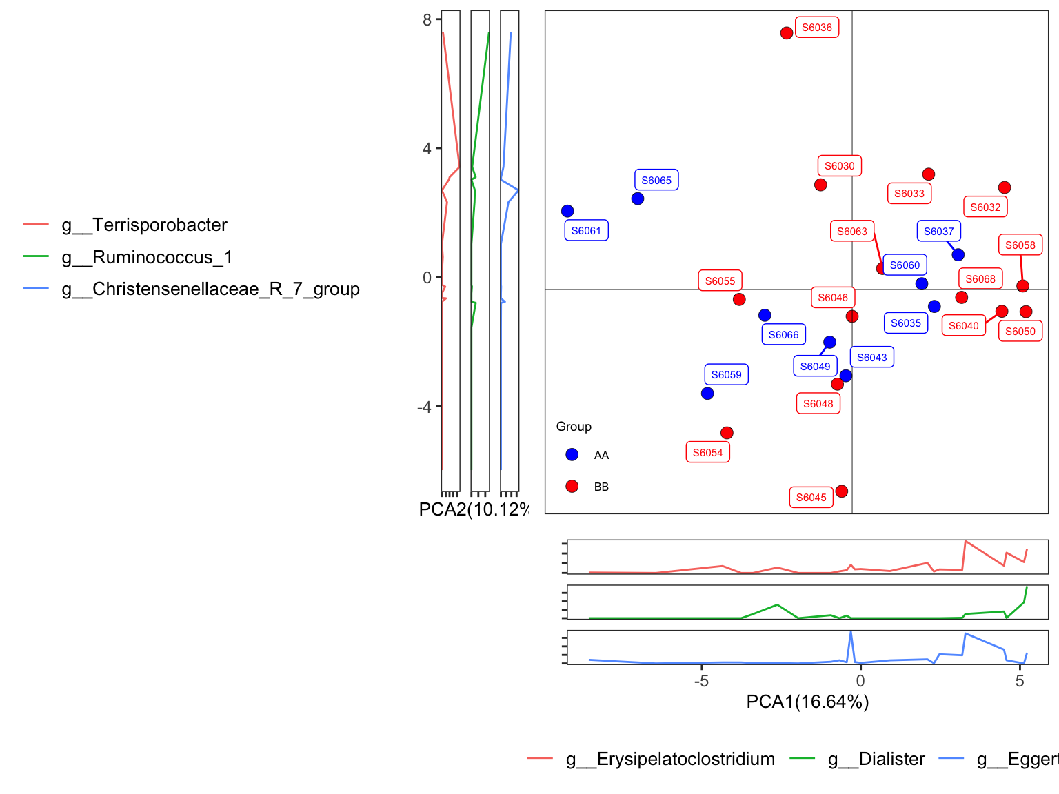
Figure 7.6: Principal Component Analysis (PCA): Ordinary pattern with SampleID
- biplot with topN dominant taxa
plot_ggbiplot(ResultList = ordination_PCA,
              group = "Group",
              group_color = c("blue", "red"),
              topN = 5,
              ellipse = TRUE,
              labels = "SampleID")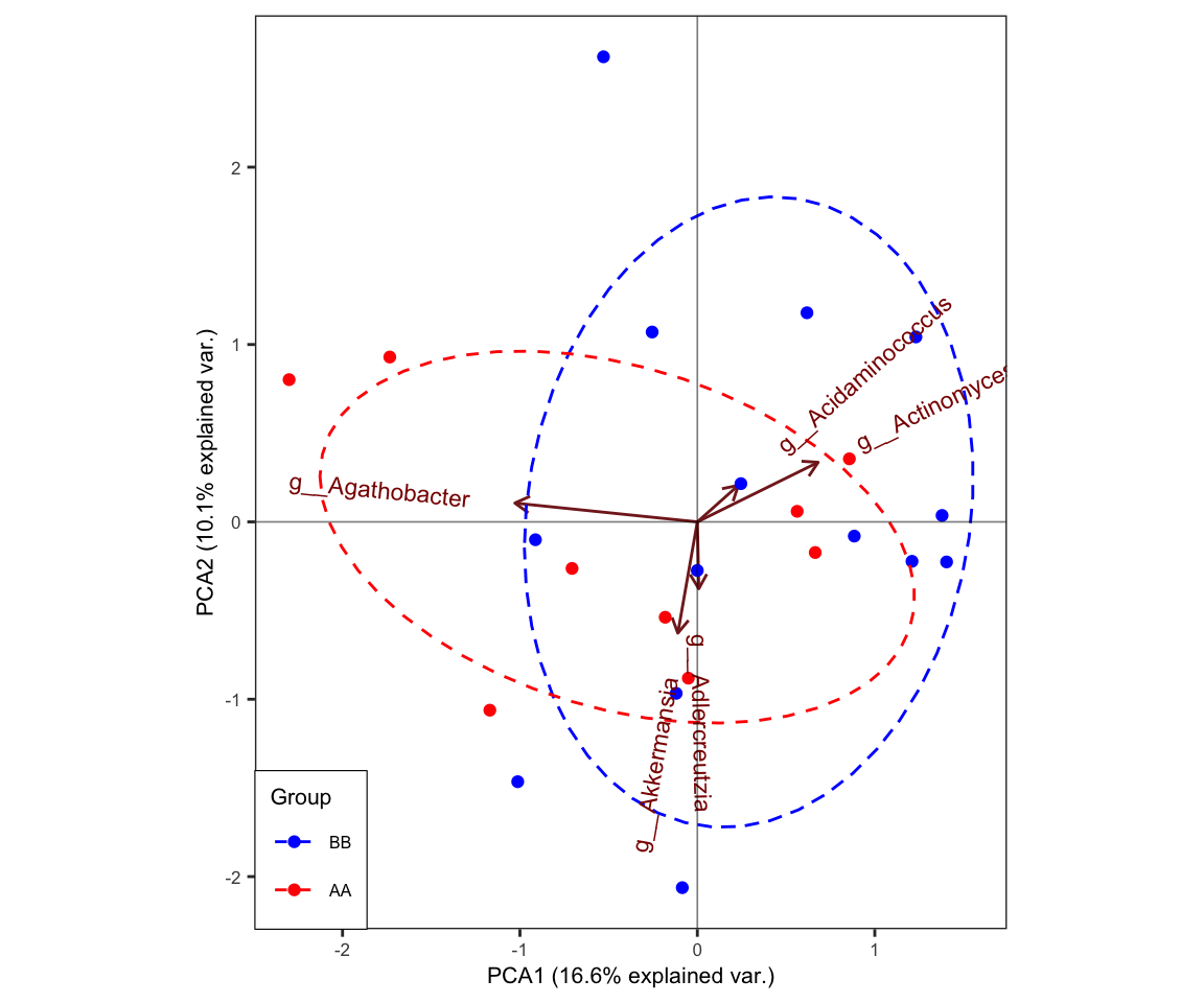
Figure 7.7: Principal Component Analysis (PCA): biplot
biplot not only shows the distribution of samples, but also displays correlation among the dominant taxa. We chose top 5 dominant taxa.
The length of vector approximates standard deviation of variables (bacteria); the angles between variables (bacteria in this case) reflect their correlations: the cosine of angle approximates correlation between variables (bacteria).
7.10.2 Principal Coordinate Analysis (PCoA)
Principal Coordinate Analysis (PCoA) could use different distance measures (e.g., Jaccard, Bray-Curtis, Euclidean, etc.) as input for ordination, but pay attention to the data matrix with negative values (not suitable for Bray-Curtis distance).
As PCA, PCoA uses eigenvalues to measure the importance of a set of returned orthogonal axes. The dimensionality of matrix is reduced by determining each eigenvector and eigenvalue. The principal coordinates are obtained by scaling each eigenvector.
7.10.2.1 Running PCoA
Different distance measures could be affected by different factors (eg, low abundance taxa for Bary Curtis distance), so we recommend users taking care for whether performing the preprocess before calculating the distance. Here, we coincided to the tactics of the PCA analysis.
ordination_PCoA <- run_ordination(
                       ps = dada2_ps_genus_filter_trim,
                       group = "Group",
                       method = "PCoA")
names(ordination_PCoA)
## [1] "fit" "dat" "explains" "eigvalue" "PERMANOVA" "BETADISPER" "axis_taxa_cor"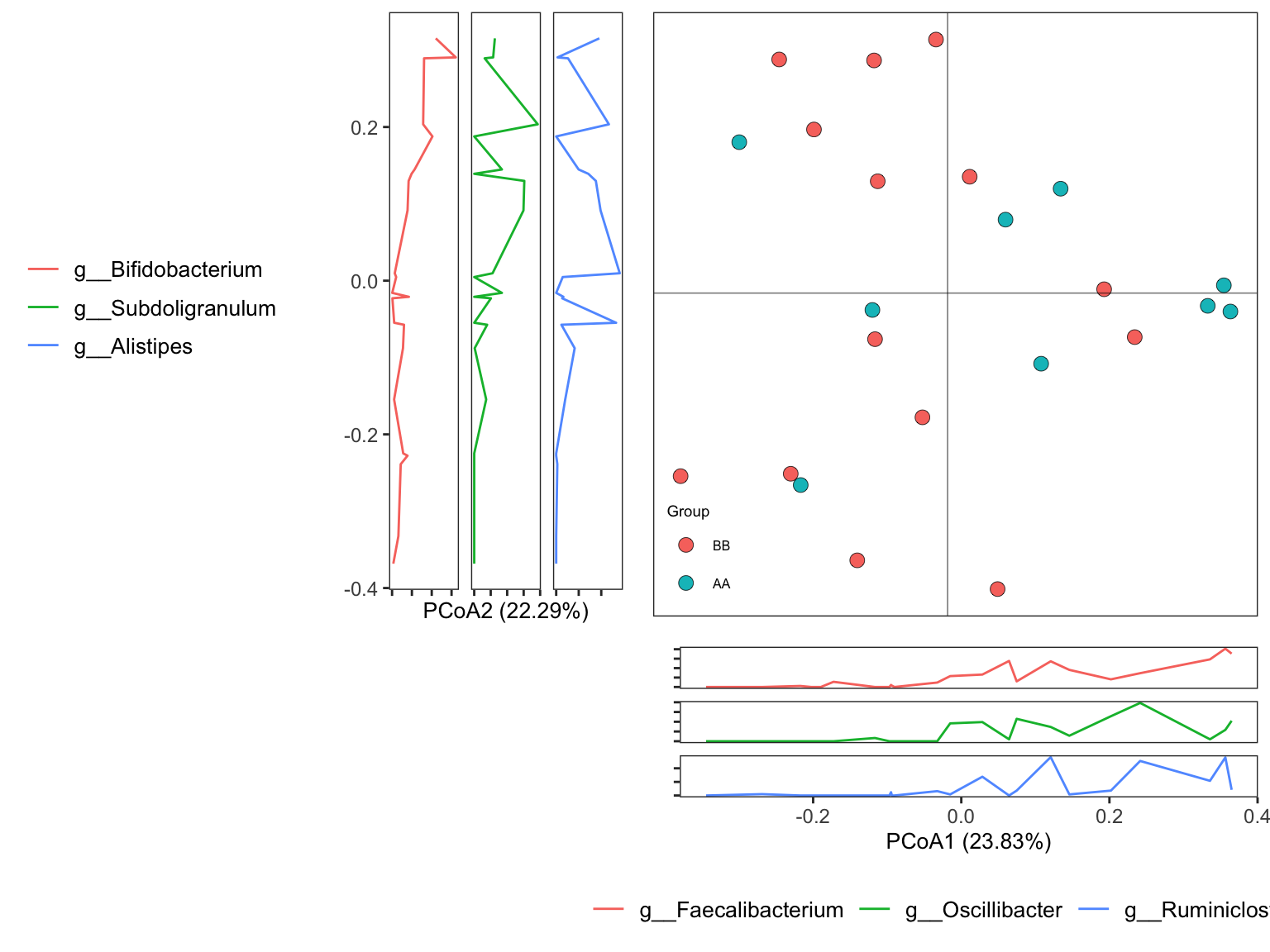
7.10.3 t-distributed stochastic neighbor embedding (t-SNE)
t-distributed stochastic neighbor embedding (t-SNE) is a statistical method for visualizing high-dimensional data by giving each datapoint a location in a two or three-dimensional map. It is based on Stochastic Neighbor Embedding originally developed by Sam Roweis and Geoffrey Hinton, where Laurens van der Maaten proposed the t-distributed variant. It is a nonlinear dimensionality reduction technique well-suited for embedding high-dimensional data for visualization in a low-dimensional space of two or three dimensions. Specifically, it models each high-dimensional object by a two- or three-dimensional point in such a way that similar objects are modeled by nearby points and dissimilar objects are modeled by distant points with high probability.
7.10.3.1 Running tSNE
Perplexity parameter is for how many neighbors to be chosen.
ordination_tSNE <- run_ordination(
                       ps = dada2_ps_genus_filter_trim,
                       group = "Group",
                       method = "tSNE",
                       para =list(Perplexity=2))

names(ordination_tSNE)
## [1] "fit" "dat" "explains" "eigvalue" "PERMANOVA" "BETADISPER" "axis_taxa_cor"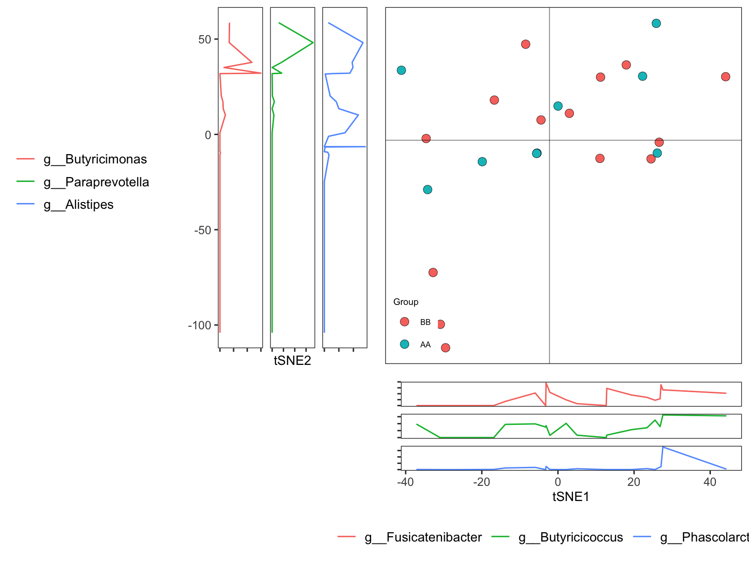
7.10.4 Uniform Manifold Approximation and Projection for Dimension Reduction (UMAP)
Uniform Manifold Approximation and Projection (UMAP) (McInnes et al. 2022) is a dimension reduction technique that can be used for visualisation similarly to t-SNE, but also for general non-linear dimension reduction. The algorithm is founded on three assumptions about the data.
7.10.4.1 Running UMAP
ordination_UMAP <- run_ordination(
                       ps = dada2_ps_genus_filter_trim,
                       group = "Group",
                       method = "UMAP")

names(ordination_UMAP)
## [1] "fit" "dat" "explains" "eigvalue" "PERMANOVA" "BETADISPER" "axis_taxa_cor"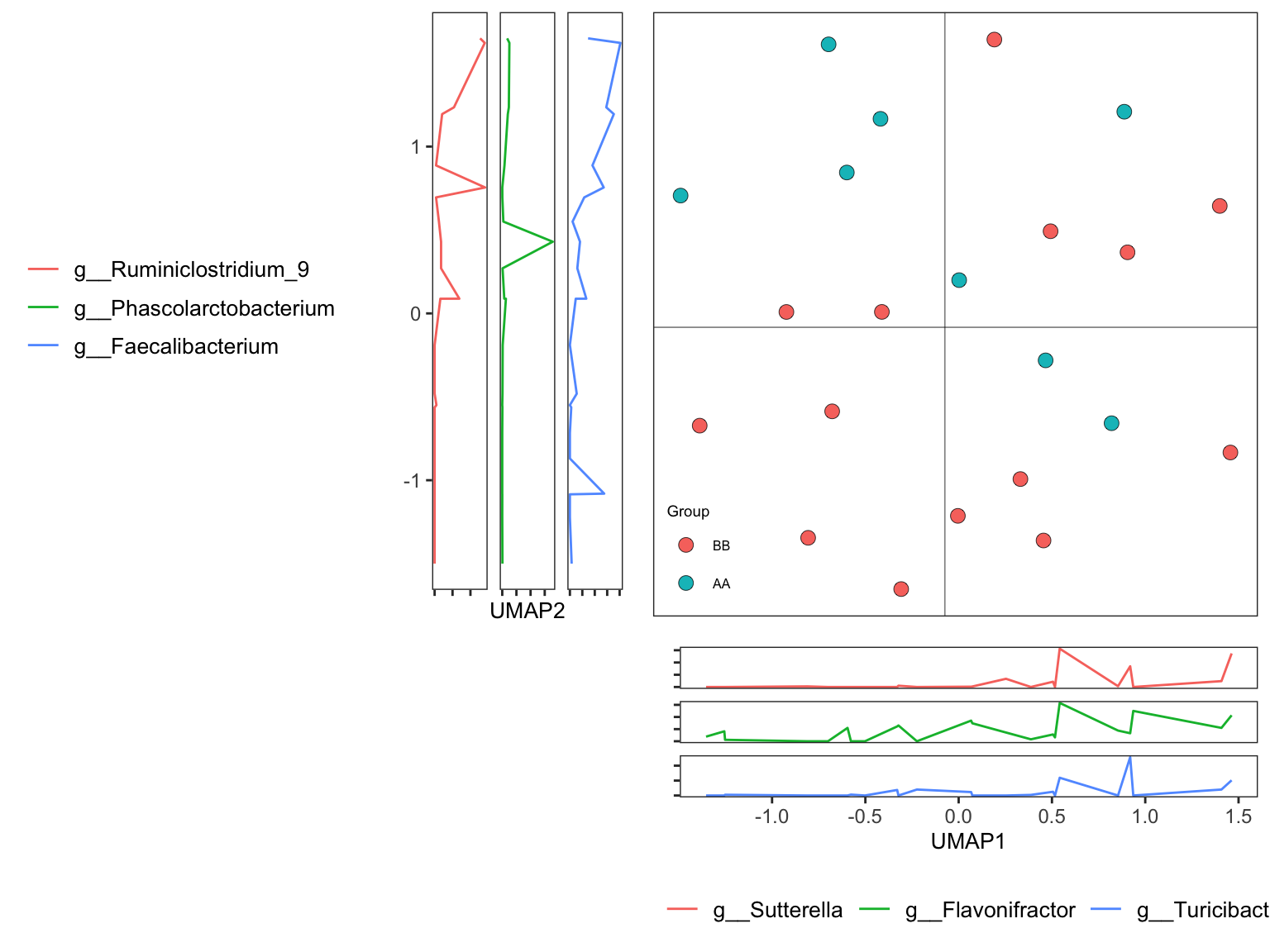
7.11 Systematic Information
## ─ Session info ───────────────────────────────────────────────────────────────────────────────────────────────────────────────────────────
##  setting  value
##  version  R version 4.1.3 (2022-03-10)
##  os       macOS Monterey 12.2.1
##  system   x86_64, darwin17.0
##  ui       RStudio
##  language (EN)
##  collate  en_US.UTF-8
##  ctype    en_US.UTF-8
##  tz       Asia/Shanghai
##  date     2023-11-30
##  rstudio  2023.09.0+463 Desert Sunflower (desktop)
##  pandoc   3.1.1 @ /Applications/RStudio.app/Contents/Resources/app/quarto/bin/tools/ (via rmarkdown)
##
## ─ Packages ───────────────────────────────────────────────────────────────────────────────────────────────────────────────────────────────
##  package              * version   date (UTC) lib source
##  abind                  1.4-5     2016-07-21 [2] CRAN (R 4.1.0)
##  ade4                   1.7-22    2023-02-06 [2] CRAN (R 4.1.2)
##  annotate               1.72.0    2021-10-26 [2] Bioconductor
##  AnnotationDbi          1.60.2    2023-03-10 [2] Bioconductor
##  ape                  * 5.7-1     2023-03-13 [2] CRAN (R 4.1.2)
##  askpass                1.1       2019-01-13 [2] CRAN (R 4.1.0)
##  backports              1.4.1     2021-12-13 [2] CRAN (R 4.1.0)
##  base64enc              0.1-3     2015-07-28 [2] CRAN (R 4.1.0)
##  Biobase                2.54.0    2021-10-26 [2] Bioconductor
##  BiocGenerics           0.40.0    2021-10-26 [2] Bioconductor
##  BiocParallel           1.28.3    2021-12-09 [2] Bioconductor
##  biomformat             1.22.0    2021-10-26 [2] Bioconductor
##  Biostrings             2.62.0    2021-10-26 [2] Bioconductor
##  bit                    4.0.5     2022-11-15 [2] CRAN (R 4.1.2)
##  bit64                  4.0.5     2020-08-30 [2] CRAN (R 4.1.0)
##  bitops                 1.0-7     2021-04-24 [2] CRAN (R 4.1.0)
##  blob                   1.2.4     2023-03-17 [2] CRAN (R 4.1.2)
##  bookdown               0.34      2023-05-09 [2] CRAN (R 4.1.2)
##  broom                  1.0.5     2023-06-09 [2] CRAN (R 4.1.3)
##  bslib                  0.6.0     2023-11-21 [1] CRAN (R 4.1.3)
##  cachem                 1.0.8     2023-05-01 [2] CRAN (R 4.1.2)
##  callr                  3.7.3     2022-11-02 [2] CRAN (R 4.1.2)
##  car                    3.1-2     2023-03-30 [2] CRAN (R 4.1.2)
##  carData                3.0-5     2022-01-06 [2] CRAN (R 4.1.2)
##  caTools                1.18.2    2021-03-28 [2] CRAN (R 4.1.0)
##  checkmate              2.2.0     2023-04-27 [2] CRAN (R 4.1.2)
##  cli                    3.6.1     2023-03-23 [2] CRAN (R 4.1.2)
##  cluster                2.1.4     2022-08-22 [2] CRAN (R 4.1.2)
##  coda                   0.19-4    2020-09-30 [2] CRAN (R 4.1.0)
##  codetools              0.2-19    2023-02-01 [2] CRAN (R 4.1.2)
##  coin                   1.4-2     2021-10-08 [2] CRAN (R 4.1.0)
##  colorspace             2.1-0     2023-01-23 [2] CRAN (R 4.1.2)
##  conflicted           * 1.2.0     2023-02-01 [2] CRAN (R 4.1.2)
##  corrplot               0.92      2021-11-18 [2] CRAN (R 4.1.0)
##  cowplot                1.1.1     2020-12-30 [2] CRAN (R 4.1.0)
##  crayon                 1.5.2     2022-09-29 [2] CRAN (R 4.1.2)
##  crosstalk              1.2.0     2021-11-04 [2] CRAN (R 4.1.0)
##  data.table             1.14.8    2023-02-17 [2] CRAN (R 4.1.2)
##  DBI                    1.1.3     2022-06-18 [2] CRAN (R 4.1.2)
##  DelayedArray           0.20.0    2021-10-26 [2] Bioconductor
##  DESeq2                 1.34.0    2021-10-26 [2] Bioconductor
##  devtools               2.4.5     2022-10-11 [2] CRAN (R 4.1.2)
##  digest                 0.6.33    2023-07-07 [1] CRAN (R 4.1.3)
##  dplyr                * 1.1.2     2023-04-20 [2] CRAN (R 4.1.2)
##  DT                     0.28      2023-05-18 [2] CRAN (R 4.1.3)
##  edgeR                  3.36.0    2021-10-26 [2] Bioconductor
##  ellipsis               0.3.2     2021-04-29 [2] CRAN (R 4.1.0)
##  emmeans                1.8.7     2023-06-23 [1] CRAN (R 4.1.3)
##  estimability           1.4.1     2022-08-05 [2] CRAN (R 4.1.2)
##  evaluate               0.21      2023-05-05 [2] CRAN (R 4.1.2)
##  FactoMineR             2.8       2023-03-27 [2] CRAN (R 4.1.2)
##  fansi                  1.0.4     2023-01-22 [2] CRAN (R 4.1.2)
##  farver                 2.1.1     2022-07-06 [2] CRAN (R 4.1.2)
##  fastmap                1.1.1     2023-02-24 [2] CRAN (R 4.1.2)
##  flashClust             1.01-2    2012-08-21 [2] CRAN (R 4.1.0)
##  foreach                1.5.2     2022-02-02 [2] CRAN (R 4.1.2)
##  foreign                0.8-84    2022-12-06 [2] CRAN (R 4.1.2)
##  Formula                1.2-5     2023-02-24 [2] CRAN (R 4.1.2)
##  fs                     1.6.2     2023-04-25 [2] CRAN (R 4.1.2)
##  genefilter             1.76.0    2021-10-26 [2] Bioconductor
##  geneplotter            1.72.0    2021-10-26 [2] Bioconductor
##  generics               0.1.3     2022-07-05 [2] CRAN (R 4.1.2)
##  GenomeInfoDb           1.30.1    2022-01-30 [2] Bioconductor
##  GenomeInfoDbData       1.2.7     2022-03-09 [2] Bioconductor
##  GenomicRanges          1.46.1    2021-11-18 [2] Bioconductor
##  ggplot2              * 3.4.2     2023-04-03 [2] CRAN (R 4.1.2)
##  ggpubr               * 0.6.0     2023-02-10 [2] CRAN (R 4.1.2)
##  ggrepel                0.9.3     2023-02-03 [2] CRAN (R 4.1.2)
##  ggsci                  3.0.0     2023-03-08 [2] CRAN (R 4.1.2)
##  ggsignif               0.6.4     2022-10-13 [2] CRAN (R 4.1.2)
##  glmnet                 4.1-7     2023-03-23 [2] CRAN (R 4.1.2)
##  glue                   1.6.2     2022-02-24 [2] CRAN (R 4.1.2)
##  gplots                 3.1.3     2022-04-25 [2] CRAN (R 4.1.2)
##  gridExtra              2.3       2017-09-09 [2] CRAN (R 4.1.0)
##  gtable                 0.3.3     2023-03-21 [2] CRAN (R 4.1.2)
##  gtools                 3.9.4     2022-11-27 [2] CRAN (R 4.1.2)
##  highr                  0.10      2022-12-22 [2] CRAN (R 4.1.2)
##  Hmisc                  5.1-0     2023-05-08 [2] CRAN (R 4.1.2)
##  htmlTable              2.4.1     2022-07-07 [2] CRAN (R 4.1.2)
##  htmltools              0.5.7     2023-11-03 [1] CRAN (R 4.1.3)
##  htmlwidgets            1.6.2     2023-03-17 [2] CRAN (R 4.1.2)
##  httpuv                 1.6.11    2023-05-11 [2] CRAN (R 4.1.3)
##  httr                   1.4.6     2023-05-08 [2] CRAN (R 4.1.2)
##  igraph                 1.5.0     2023-06-16 [1] CRAN (R 4.1.3)
##  IRanges                2.28.0    2021-10-26 [2] Bioconductor
##  iterators              1.0.14    2022-02-05 [2] CRAN (R 4.1.2)
##  jquerylib              0.1.4     2021-04-26 [2] CRAN (R 4.1.0)
##  jsonlite               1.8.7     2023-06-29 [2] CRAN (R 4.1.3)
##  kableExtra             1.3.4     2021-02-20 [2] CRAN (R 4.1.2)
##  KEGGREST               1.34.0    2021-10-26 [2] Bioconductor
##  KernSmooth             2.23-22   2023-07-10 [2] CRAN (R 4.1.3)
##  knitr                  1.43      2023-05-25 [2] CRAN (R 4.1.3)
##  labeling               0.4.2     2020-10-20 [2] CRAN (R 4.1.0)
##  later                  1.3.1     2023-05-02 [2] CRAN (R 4.1.2)
##  lattice              * 0.21-8    2023-04-05 [2] CRAN (R 4.1.2)
##  leaps                  3.1       2020-01-16 [2] CRAN (R 4.1.0)
##  libcoin                1.0-9     2021-09-27 [2] CRAN (R 4.1.0)
##  lifecycle              1.0.3     2022-10-07 [2] CRAN (R 4.1.2)
##  limma                  3.50.3    2022-04-07 [2] Bioconductor
##  locfit                 1.5-9.8   2023-06-11 [2] CRAN (R 4.1.3)
##  magrittr               2.0.3     2022-03-30 [2] CRAN (R 4.1.2)
##  MASS                   7.3-60    2023-05-04 [2] CRAN (R 4.1.2)
##  Matrix                 1.6-0     2023-07-08 [2] CRAN (R 4.1.3)
##  MatrixGenerics         1.6.0     2021-10-26 [2] Bioconductor
##  matrixStats            1.0.0     2023-06-02 [2] CRAN (R 4.1.3)
##  memoise                2.0.1     2021-11-26 [2] CRAN (R 4.1.0)
##  metagenomeSeq          1.36.0    2021-10-26 [2] Bioconductor
##  mgcv                   1.8-42    2023-03-02 [2] CRAN (R 4.1.2)
##  microbiome             1.16.0    2021-10-26 [2] Bioconductor
##  mime                   0.12      2021-09-28 [2] CRAN (R 4.1.0)
##  miniUI                 0.1.1.1   2018-05-18 [2] CRAN (R 4.1.0)
##  modeltools             0.2-23    2020-03-05 [2] CRAN (R 4.1.0)
##  multcomp               1.4-25    2023-06-20 [2] CRAN (R 4.1.3)
##  multcompView           0.1-9     2023-04-09 [2] CRAN (R 4.1.2)
##  multtest               2.50.0    2021-10-26 [2] Bioconductor
##  munsell                0.5.0     2018-06-12 [2] CRAN (R 4.1.0)
##  mvtnorm                1.2-2     2023-06-08 [2] CRAN (R 4.1.3)
##  nlme                 * 3.1-162   2023-01-31 [2] CRAN (R 4.1.2)
##  nnet                   7.3-19    2023-05-03 [2] CRAN (R 4.1.2)
##  openssl                2.0.6     2023-03-09 [2] CRAN (R 4.1.2)
##  permute              * 0.9-7     2022-01-27 [2] CRAN (R 4.1.2)
##  phyloseq             * 1.38.0    2021-10-26 [2] Bioconductor
##  picante              * 1.8.2     2020-06-10 [2] CRAN (R 4.1.0)
##  pillar                 1.9.0     2023-03-22 [2] CRAN (R 4.1.2)
##  pkgbuild               1.4.2     2023-06-26 [2] CRAN (R 4.1.3)
##  pkgconfig              2.0.3     2019-09-22 [2] CRAN (R 4.1.0)
##  pkgload                1.3.2.1   2023-07-08 [2] CRAN (R 4.1.3)
##  plyr                   1.8.8     2022-11-11 [2] CRAN (R 4.1.2)
##  png                    0.1-8     2022-11-29 [2] CRAN (R 4.1.2)
##  prettyunits            1.1.1     2020-01-24 [2] CRAN (R 4.1.0)
##  processx               3.8.2     2023-06-30 [2] CRAN (R 4.1.3)
##  profvis                0.3.8     2023-05-02 [2] CRAN (R 4.1.2)
##  promises               1.2.0.1   2021-02-11 [2] CRAN (R 4.1.0)
##  ps                     1.7.5     2023-04-18 [2] CRAN (R 4.1.2)
##  purrr                  1.0.1     2023-01-10 [2] CRAN (R 4.1.2)
##  R6                     2.5.1     2021-08-19 [2] CRAN (R 4.1.0)
##  RColorBrewer           1.1-3     2022-04-03 [2] CRAN (R 4.1.2)
##  Rcpp                   1.0.11    2023-07-06 [1] CRAN (R 4.1.3)
##  RCurl                  1.98-1.12 2023-03-27 [2] CRAN (R 4.1.2)
##  remotes                2.4.2     2021-11-30 [2] CRAN (R 4.1.0)
##  reshape2               1.4.4     2020-04-09 [2] CRAN (R 4.1.0)
##  reticulate             1.30      2023-06-09 [2] CRAN (R 4.1.3)
##  rhdf5                  2.38.1    2022-03-10 [2] Bioconductor
##  rhdf5filters           1.6.0     2021-10-26 [2] Bioconductor
##  Rhdf5lib               1.16.0    2021-10-26 [2] Bioconductor
##  rlang                  1.1.1     2023-04-28 [1] CRAN (R 4.1.2)
##  rmarkdown              2.23      2023-07-01 [2] CRAN (R 4.1.3)
##  rpart                  4.1.19    2022-10-21 [2] CRAN (R 4.1.2)
##  RSpectra               0.16-1    2022-04-24 [2] CRAN (R 4.1.2)
##  RSQLite                2.3.1     2023-04-03 [2] CRAN (R 4.1.2)
##  rstatix                0.7.2     2023-02-01 [2] CRAN (R 4.1.2)
##  rstudioapi             0.15.0    2023-07-07 [2] CRAN (R 4.1.3)
##  Rtsne                  0.16      2022-04-17 [2] CRAN (R 4.1.2)
##  rvest                  1.0.3     2022-08-19 [2] CRAN (R 4.1.2)
##  S4Vectors              0.32.4    2022-03-29 [2] Bioconductor
##  sandwich               3.0-2     2022-06-15 [2] CRAN (R 4.1.2)
##  sass                   0.4.6     2023-05-03 [2] CRAN (R 4.1.2)
##  scales                 1.2.1     2022-08-20 [2] CRAN (R 4.1.2)
##  scatterplot3d          0.3-44    2023-05-05 [2] CRAN (R 4.1.2)
##  sessioninfo            1.2.2     2021-12-06 [2] CRAN (R 4.1.0)
##  shape                  1.4.6     2021-05-19 [2] CRAN (R 4.1.0)
##  shiny                  1.7.4.1   2023-07-06 [2] CRAN (R 4.1.3)
##  stringi                1.7.12    2023-01-11 [2] CRAN (R 4.1.2)
##  stringr                1.5.0     2022-12-02 [2] CRAN (R 4.1.2)
##  SummarizedExperiment   1.24.0    2021-10-26 [2] Bioconductor
##  survival               3.5-5     2023-03-12 [2] CRAN (R 4.1.2)
##  svglite                2.1.1     2023-01-10 [2] CRAN (R 4.1.2)
##  systemfonts            1.0.4     2022-02-11 [2] CRAN (R 4.1.2)
##  TH.data                1.1-2     2023-04-17 [2] CRAN (R 4.1.2)
##  tibble               * 3.2.1     2023-03-20 [2] CRAN (R 4.1.2)
##  tidyr                  1.3.0     2023-01-24 [2] CRAN (R 4.1.2)
##  tidyselect             1.2.0     2022-10-10 [2] CRAN (R 4.1.2)
##  umap                   0.2.10.0  2023-02-01 [2] CRAN (R 4.1.2)
##  urlchecker             1.0.1     2021-11-30 [2] CRAN (R 4.1.0)
##  usethis                2.2.2     2023-07-06 [2] CRAN (R 4.1.3)
##  utf8                   1.2.3     2023-01-31 [2] CRAN (R 4.1.2)
##  vctrs                  0.6.3     2023-06-14 [1] CRAN (R 4.1.3)
##  vegan                * 2.6-4     2022-10-11 [2] CRAN (R 4.1.2)
##  viridisLite            0.4.2     2023-05-02 [2] CRAN (R 4.1.2)
##  webshot                0.5.5     2023-06-26 [2] CRAN (R 4.1.3)
##  withr                  2.5.0     2022-03-03 [2] CRAN (R 4.1.2)
##  Wrench                 1.12.0    2021-10-26 [2] Bioconductor
##  xfun                   0.40      2023-08-09 [1] CRAN (R 4.1.3)
##  XMAS2                * 2.2.0     2023-11-30 [1] local
##  XML                    3.99-0.14 2023-03-19 [2] CRAN (R 4.1.2)
##  xml2                   1.3.5     2023-07-06 [2] CRAN (R 4.1.3)
##  xtable                 1.8-4     2019-04-21 [2] CRAN (R 4.1.0)
##  XVector                0.34.0    2021-10-26 [2] Bioconductor
##  yaml                   2.3.7     2023-01-23 [2] CRAN (R 4.1.2)
##  zlibbioc               1.40.0    2021-10-26 [2] Bioconductor
##  zoo                    1.8-12    2023-04-13 [2] CRAN (R 4.1.2)
##
##  [1] /Users/zouhua/Library/R/x86_64/4.1/library
##  [2] /Library/Frameworks/R.framework/Versions/4.1/Resources/library
##
## ──────────────────────────────────────────────────────────────────────────────────────────────────────────────────────────────────────────