Chapter 6 Aplha diversity
Alpha diversity is a measure of microbiome diversity applicable to a single sample. The commonly used metrics/indices are Shannon, Chao1, Observed, Simpson, Gini and Inverse Simpson. The reference of this part is (A et al. 2020).
It is important to note that, alpha diversity indices are sensitive to noise that is inherent to application of polymerase chain reaction and the sequencing errors.
Cautions: Shannon, Simpson and InvSimpson measures are both for relative or absolute abundance.
As defined by Shannon, the index of Shannon index is given as follow:
\[H^{'} = \sum_{i=1}^{S}p_{i}\,\ln\,p_{i}\] where \(p_{i}\) is the proportion of individuals (or relative abundance) of species \(i\) in the community and \(S\) is the total number of species present so that \(\sum_{i=1}^{S}p_{i} = 1\).
Outline of this Chapter:
6.2 Importing Data
data("dada2_ps")
dada2_ps_remove_BRS <- get_GroupPhyloseq(
                         ps = dada2_ps,
                         group = "Group",
                         group_names = "QC",
                         discard = TRUE)
dada2_ps_remove_BRS
## phyloseq-class experiment-level object
## otu_table() OTU Table: [ 896 taxa and 23 samples ]
## sample_data() Sample Data: [ 23 samples by 1 sample variables ]
## tax_table() Taxonomy Table: [ 896 taxa by 7 taxonomic ranks ]
## phy_tree() Phylogenetic Tree: [ 896 tips and 893 internal nodes ]
## refseq() DNAStringSet: [ 896 reference sequences ]## phyloseq-class experiment-level object
## otu_table() OTU Table: [ 3426 taxa and 34 samples ]
## sample_data() Sample Data: [ 34 samples by 8 sample variables ]
## tax_table() Taxonomy Table: [ 3426 taxa by 7 taxonomic ranks ]
## phy_tree() Phylogenetic Tree: [ 3426 tips and 3424 internal nodes ]metagenomic sequencing (metaphlan2/3)
data("metaphlan2_ps")
metaphlan2_ps_remove_BRS <- get_GroupPhyloseq(
                               ps = metaphlan2_ps,
                               group = "Group",
                               group_names = "QC",
                               discard = TRUE)
metaphlan2_ps_remove_BRS
## phyloseq-class experiment-level object
## otu_table() OTU Table: [ 326 taxa and 22 samples ]
## sample_data() Sample Data: [ 22 samples by 2 sample variables ]
## tax_table() Taxonomy Table: [ 326 taxa by 7 taxonomic ranks ]6.3 Equal sample sums
6.3.1 dada2_ps dataset
- Summary counts
The previous result from Rarefaction Curves had demonstrated that the sequence depth of each sample has a larger significance and normalizing the samples’ depth into equal sampling depth is necessary.
##    Min. 1st Qu.  Median    Mean 3rd Qu.    Max.
##   51181   58608   61435   61257   64283   71667
As is evident there is a large difference in the number of reads. Minimum is 51181 and maximum is 71667!! There is a ~1.4X difference.
- Rarefying counts
dada2_ps_rarefy <- norm_rarefy(object = dada2_ps_remove_BRS,
                               size = 51181)
summary(sample_sums(dada2_ps_rarefy))
## Min. 1st Qu. Median Mean 3rd Qu. Max.
## 51181 51181 51181 51181 51181 51181- Checking taxa prevalence
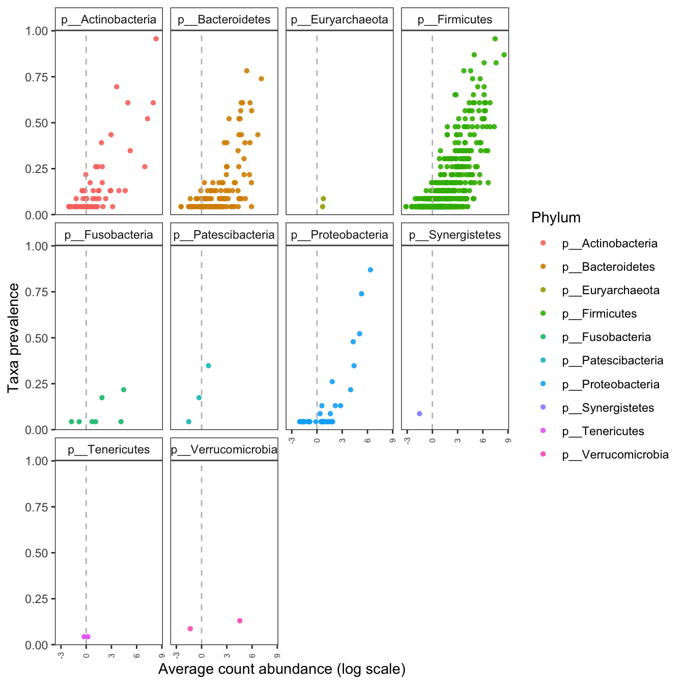
Figure 6.1: Taxa prevalence after rarefying
6.3.2 amplicon_ps dataset
- Preparing for input phyloseq object
##    Min. 1st Qu.  Median    Mean 3rd Qu.    Max.
##    1114    2139    4965    5357    8438   11449
As is evident there is a large difference in the number of reads. Minimum is 1114 and maximum is 11449!! There is a ~10X difference!
amplicon_ps_rarefy <- norm_rarefy(object = amplicon_ps,
                                  size = 1114)
summary(sample_sums(amplicon_ps))
## Min. 1st Qu. Median Mean 3rd Qu. Max.
## 1114 2139 4965 5357 8438 114496.4 Non-phylogenetic diversities
6.4.1 XMAS2 R package
- Calculation
amplicon_ps_rarefy_alpha <- run_alpha_diversity(ps = amplicon_ps_rarefy,
                                                measures = c("Shannon", "Chao1", "Observed"))
head(amplicon_ps_rarefy_alpha)
## TempRowNames SampleType Year Month Day Subject ReportedAntibioticUsage DaysSinceExperimentStart Description Observed Chao1
## 1 L1S140 gut 2008 10 28 2 Yes 0 2_Fece_10_28_2008 27 74.50
## 2 L1S208 gut 2009 1 20 2 No 84 2_Fece_1_20_2009 40 148.75
## 3 L1S8 gut 2008 10 28 1 Yes 0 1_Fece_10_28_2008 19 54.00
## 4 L1S281 gut 2009 4 14 2 No 168 2_Fece_4_14_2009 60 256.00
## 5 L3S242 right palm 2008 10 28 1 Yes 0 1_R_Palm_10_28_2008 16 42.00
## 6 L2S309 left palm 2009 1 20 2 No 84 2_L_Palm_1_20_2009 12 57.00
## se.chao1 Shannon
## 1 30.70970 3.126005
## 2 62.86107 3.303186
## 3 25.57190 2.688337
## 4 93.42352 3.664947
## 5 19.97805 2.692311
## 6 30.06061 2.082828MGS Non-phylogenetic diversities
metaphlan2_ps_alpha <- run_alpha_diversity(ps = metaphlan2_ps_remove_BRS,
                                           measures = "Shannon")
head(metaphlan2_ps_alpha)
## TempRowNames Group phynotype Shannon
## 1 s1 BB 0.00 2.876002
## 2 s2 AA 2.50 2.045392
## 3 s3 BB 0.00 3.441176
## 4 s4 AA 1.25 2.746917
## 5 s5 AA 30.00 1.450722
## 6 s6 AA 15.00 2.619951- Visualization
- single measure
plot_boxplot(data = amplicon_ps_rarefy_alpha,
             y_index = "Shannon",
             group = "SampleType",
             group_names = NULL,
             group_color = NULL,
             do_test = TRUE,
             ref_group = NULL,
             method = "wilcox.test",
             outlier = TRUE)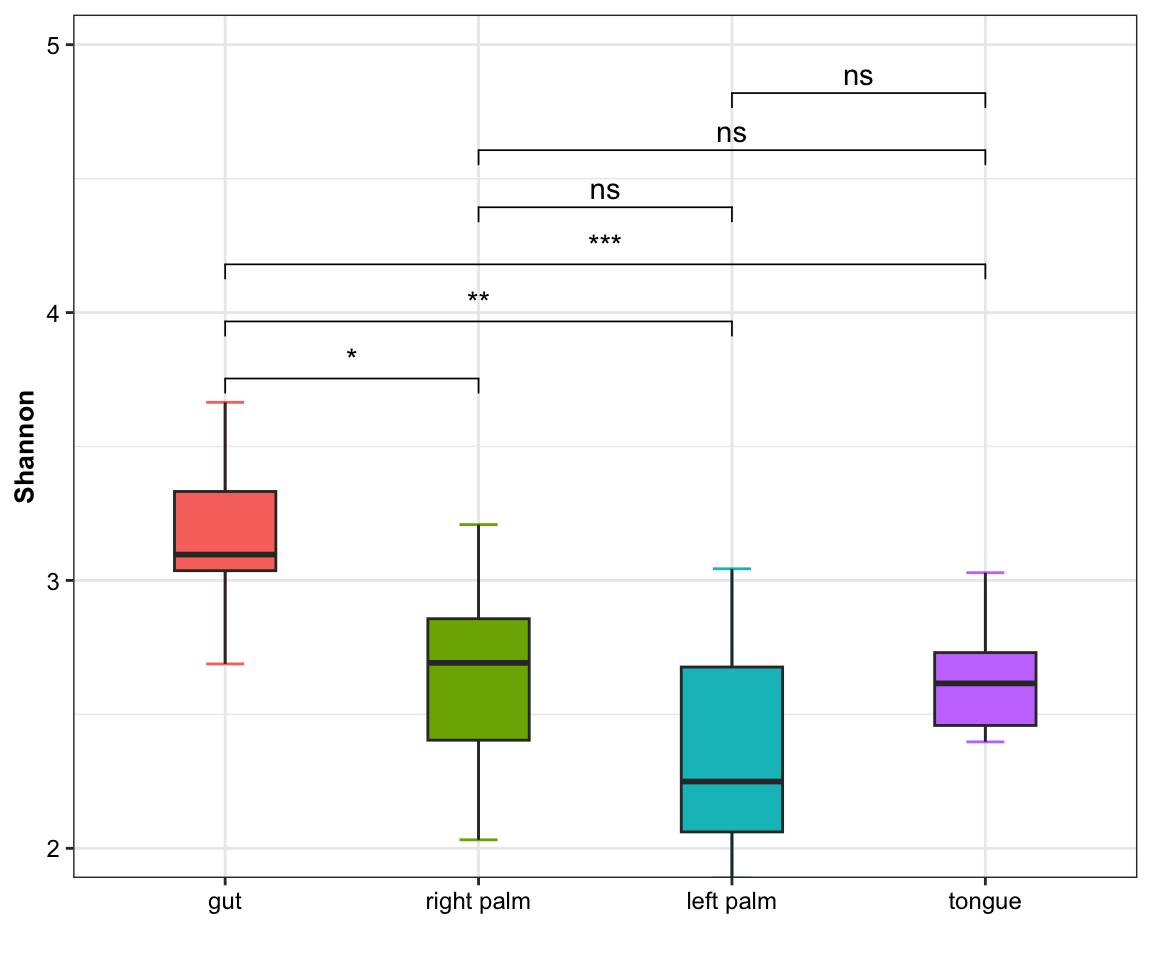
Figure 6.2: Alpha diversity from XMAS(one measure)
- multiple measures
plot_boxplot(data = amplicon_ps_rarefy_alpha,
             y_index = c("Shannon", "Chao1", "Observed"),
             group = "SampleType",
             group_names = c("gut", "right palm", "tongue"),
             group_color = c("red", "green", "blue"),
             do_test = TRUE,
             ref_group = "gut",
             method = "wilcox.test",
             outlier = TRUE)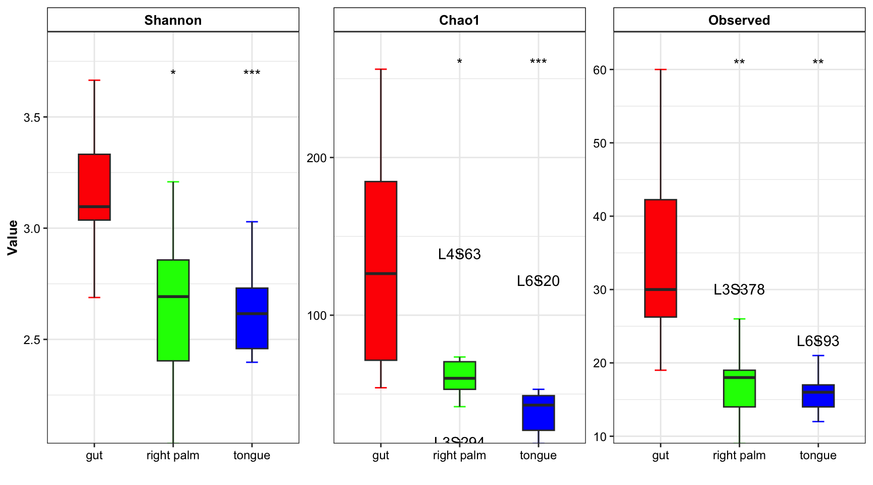
Figure 6.3: Alpha diversity from XMAS(multiple measures)
6.4.2 microbiome R package
- Calculation
amplicon_ps_rarefy_alpha_v2 <- microbiome::alpha(x = amplicon_ps_rarefy, index = "all")
DT::datatable(amplicon_ps_rarefy_alpha_v2)- Visualization
amplicon_ps_rarefy_metadata <- phyloseq::sample_data(amplicon_ps_rarefy) %>%
  data.frame()
amplicon_ps_rarefy_alpha_v2$SampleID <- rownames(amplicon_ps_rarefy_metadata)
amplicon_ps_rarefy_metadata$SampleID <- rownames(amplicon_ps_rarefy_metadata)
dat_diversity <- dplyr::inner_join(amplicon_ps_rarefy_metadata, amplicon_ps_rarefy_alpha_v2, by = "SampleID")
dat_diversity_v2 <- dat_diversity[, c("SampleType", "diversity_inverse_simpson",
                                 "diversity_gini_simpson", "diversity_shannon",
                                 "diversity_fisher", "diversity_coverage")]

colnames(dat_diversity_v2) <- c("SampleType", "Inverse Simpson", "Gini-Simpson", "Shannon", "Fisher", "Coverage")

plotdata <- dat_diversity_v2 %>%
  tidyr::gather(key = "Variable", value = "Value", -SampleType)
groups <- unique(dat_diversity_v2$SampleType)
cmp_list <- combn(seq_along(groups), 2, simplify = FALSE, FUN = function(x) {groups[x]})
pval_sign <- list(
  cutpoints = c(0, 0.0001, 0.001, 0.01, 0.05, 0.1, 1),
  symbols = c("****", "***", "**", "*", "n.s")
)

ggboxplot(plotdata,
          x = "SampleType",
          y = "Value",
          fill = "SampleType",
          palette = "jco",
          legend= "right",
          facet.by = "Variable",
          scales = "free")+
  rotate_x_text()+
  rremove("x.text")+
  stat_compare_means(
  comparisons = cmp_list,
  label = "p.signif",
  symnum.args = pval_sign)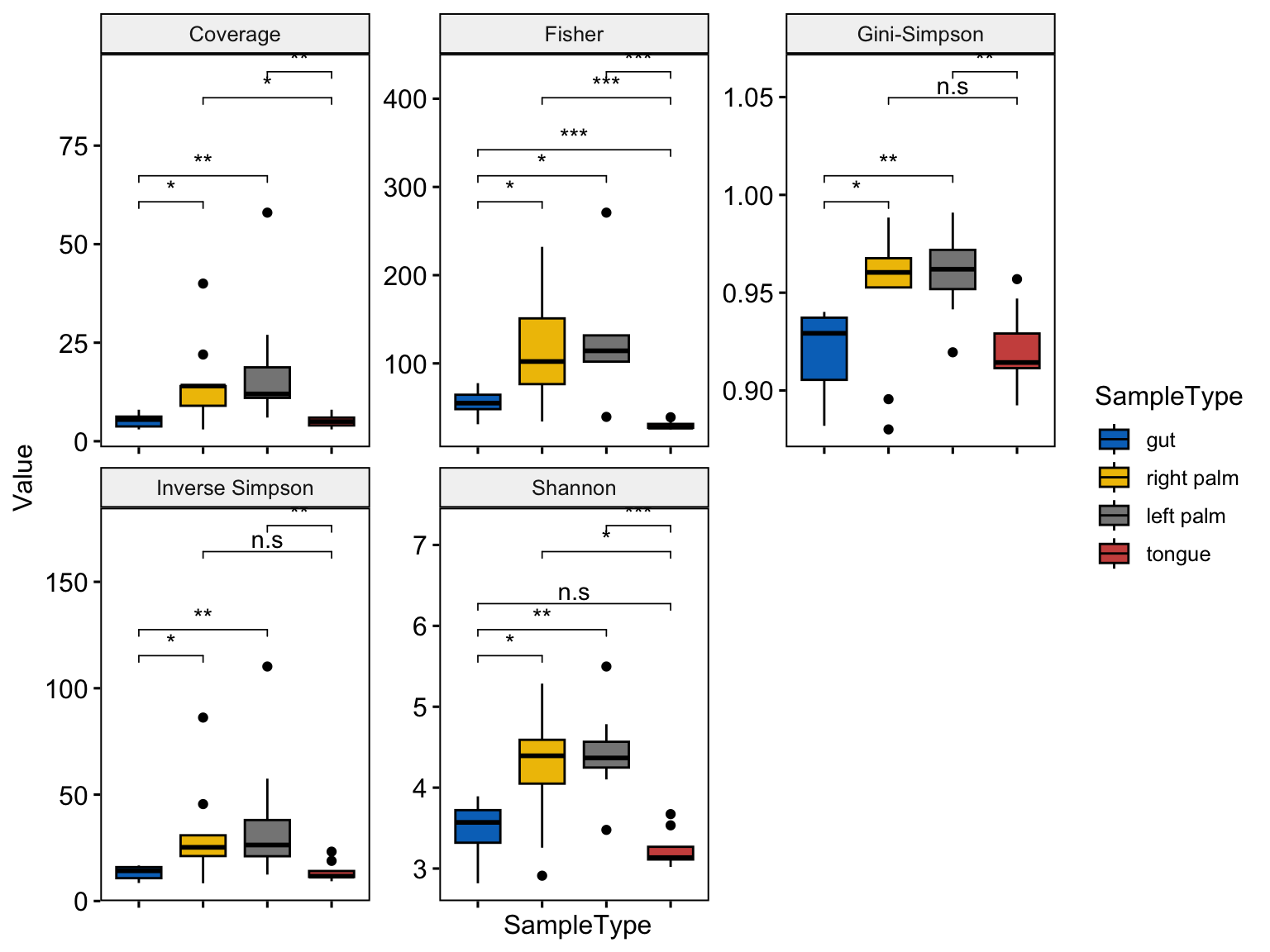
Figure 6.4: Alpha diversity from microbiome
6.5 Phylogenetic diversity
Phylogenetic diversity is calculated using the picante package.
- Calculation
library(picante)
amplicon_ps_rarefy_tab <- as.data.frame(amplicon_ps_rarefy@otu_table)
amplicon_ps_rarefy_tree <- amplicon_ps_rarefy@phy_tree
dat_pd <- pd(t(amplicon_ps_rarefy_tab),
             amplicon_ps_rarefy_tree,
             include.root = FALSE)

DT::datatable(dat_pd)- Visualization
amplicon_ps_rarefy_metadata$Phylogenetic_Diversity <- dat_pd$PD

ggboxplot(amplicon_ps_rarefy_metadata,
    x = "SampleType",
    y = "Phylogenetic_Diversity",
    fill = "SampleType",
    palette = "jco",
    ylab = "Phylogenetic Diversity",
    xlab = "Sample Type",
    legend = "right")+
  rotate_x_text()+
  stat_compare_means(
    comparisons = cmp_list,
    label = "p.signif",
    symnum.args = pval_sign)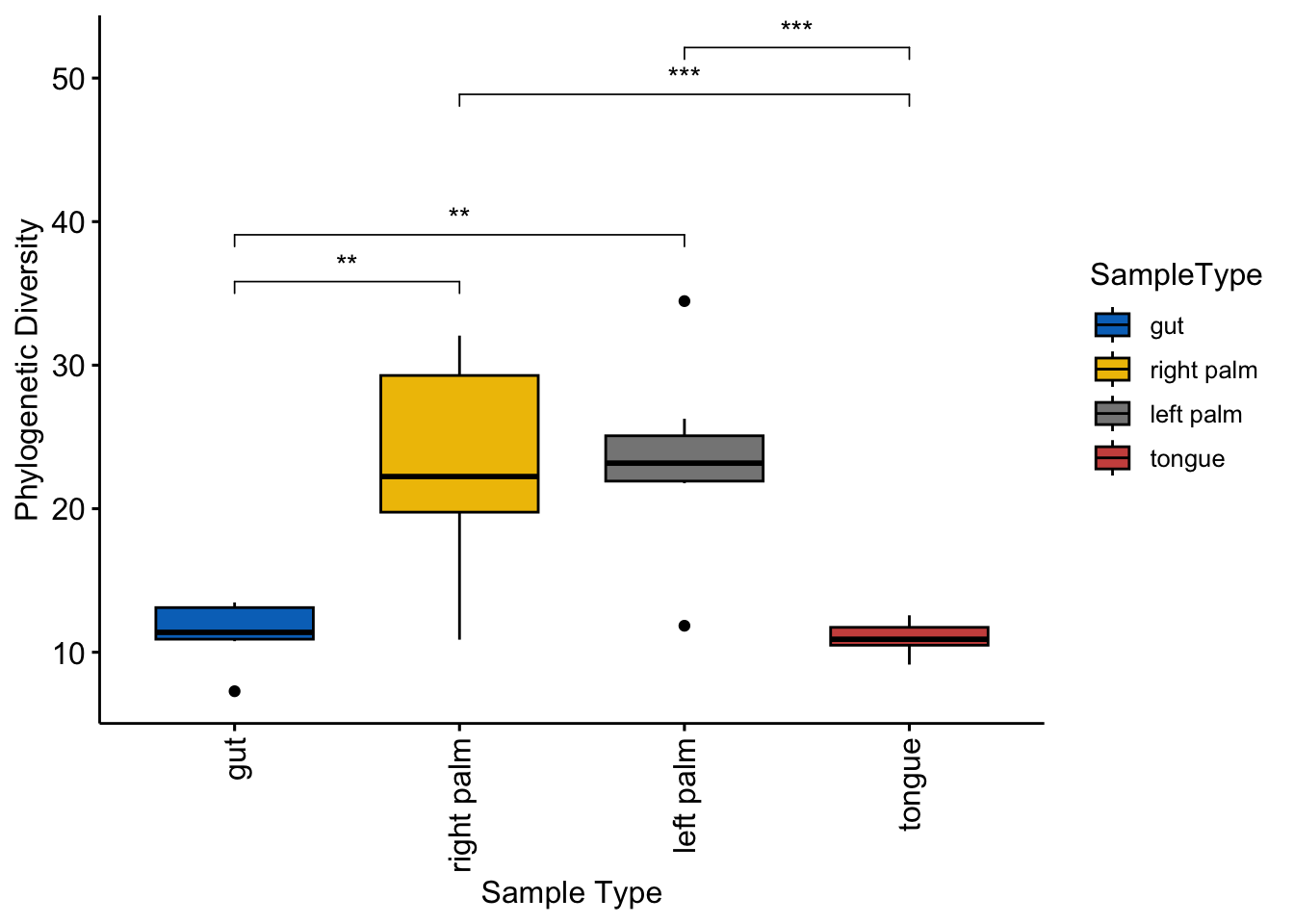
Figure 6.5: Alpha diversity from picante(Phylogenetic diversity)
Cautions:
There are arguments both for and against the use of rarefying to equal library size. The application of normalization method will depend on the type of research question. It is always good to check if there is a correlation between increasing library sizes and richness. Observed ASVs and Phylogenetic diversity can be affected by library sizes. It is always good to check for this before making a choice.
- Calculation
lib.div <- microbiome::alpha(amplicon_ps, index = "all")
lib.div2 <- microbiome::richness(amplicon_ps)
lib.div$ReadsPerSample <- sample_sums(amplicon_ps)
lib.div$Observed <- lib.div2$observed

colnames(lib.div)
## [1] "observed" "chao1" "diversity_inverse_simpson" "diversity_gini_simpson"
## [5] "diversity_shannon" "diversity_fisher" "diversity_coverage" "evenness_camargo"
## [9] "evenness_pielou" "evenness_simpson" "evenness_evar" "evenness_bulla"
## [13] "dominance_dbp" "dominance_dmn" "dominance_absolute" "dominance_relative"
## [17] "dominance_simpson" "dominance_core_abundance" "dominance_gini" "rarity_log_modulo_skewness"
## [21] "rarity_low_abundance" "rarity_rare_abundance" "ReadsPerSample" "Observed"- scatterplot
p1 <- ggscatter(lib.div, "diversity_shannon", "ReadsPerSample")+
  stat_cor(method = "pearson")

p2 <- ggscatter(lib.div, "diversity_inverse_simpson", "ReadsPerSample",dd = "loess")+
  stat_cor(method = "pearson")

p3 <- ggscatter(lib.div, "Observed", "ReadsPerSample", add = "loess") +
  stat_cor(
    method = "pearson",
    label.x = 100,
    label.y = 50000
  )

ggarrange(p1, p2, p3, ncol = 2, nrow = 2)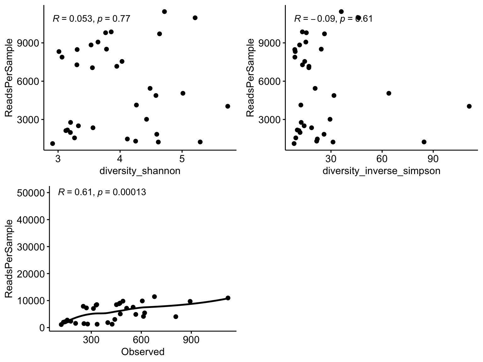
Figure 6.6: Correlation between increasing library sizes and richness
6.6 Rank Abundance
A rank abundance curve is a chart used by ecologists to display relative species abundance, a component of biodiversity. It can also be used to visualize species richness and species evenness. It overcomes the shortcomings of biodiversity indices that cannot display the relative role different variables played in their calculation. The curve is a 2D chart with relative abundance on the Y-axis and the abundance rank on the X-axis.
- X-axis: The abundance rank. The most abundant species is given rank 1, the second most abundant is 2 and so on.
- Y-axis: The relative abundance. Usually measured on a log scale, this is a measure of a species abundance (e.g., the number of individuals) relative to the abundance of other species.
plot_RankAbundance(
        ps = dada2_ps_remove_BRS,
        taxa_level = "Family",
        group = "Group",
        group_names = c("AA", "BB"))
## Successfully executed the call.## All done, quitting.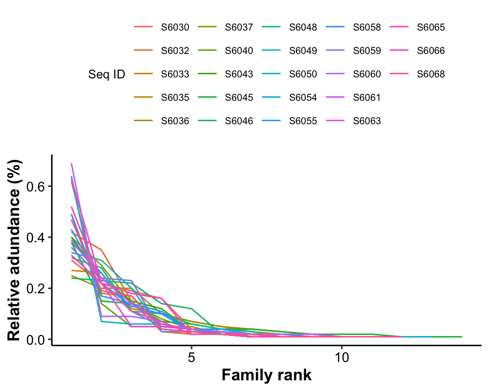
Figure 6.7: Rank Abundance
Results:
From the horizontal level (Family rank), the higher degree of width means the higher degree of Family richness;
From the vertical level (Relative abundance), the slope of the line reflects the Family evenness.
6.7 Evenness
pielou: Pielou’s evenness (Pielou, 1966), also known as Shannon or Shannon-Weaver/Wiener/Weiner evenness.
\[Pielou_{evenness} = \frac{Shannon}{log(Observed)}\]
- Calculation
amplicon_ps_rarefy_Evenness<- run_alpha_diversity(ps = amplicon_ps_rarefy,
                                                measures = "Evenness")
head(amplicon_ps_rarefy_Evenness)
## TempRowNames SampleType Year Month Day Subject ReportedAntibioticUsage DaysSinceExperimentStart Description Evenness
## 1 L1S140 gut 2008 10 28 2 Yes 0 2_Fece_10_28_2008 0.9484708
## 2 L1S208 gut 2009 1 20 2 No 84 2_Fece_1_20_2009 0.8954443
## 3 L1S8 gut 2008 10 28 1 Yes 0 1_Fece_10_28_2008 0.9130219
## 4 L1S281 gut 2009 4 14 2 No 168 2_Fece_4_14_2009 0.8951243
## 5 L3S242 right palm 2008 10 28 1 Yes 0 1_R_Palm_10_28_2008 0.9710459
## 6 L2S309 left palm 2009 1 20 2 No 84 2_L_Palm_1_20_2009 0.8381918- visualization
plot_boxplot(data = amplicon_ps_rarefy_Evenness,
             y_index = "Evenness",
             group = "SampleType",
             group_names = NULL,
             group_color = NULL,
             do_test = TRUE,
             ref_group = NULL,
             method = "wilcox.test",
             outlier = TRUE,
             group_number = TRUE)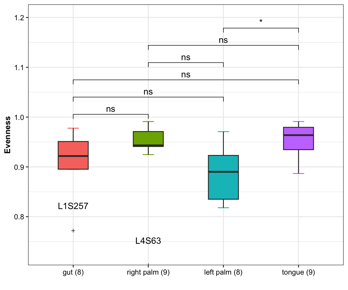
Figure 6.8: Evenness
6.8 Systematic Information
## ─ Session info ───────────────────────────────────────────────────────────────────────────────────────────────────────────────────────────
##  setting  value
##  version  R version 4.1.3 (2022-03-10)
##  os       macOS Monterey 12.2.1
##  system   x86_64, darwin17.0
##  ui       RStudio
##  language (EN)
##  collate  en_US.UTF-8
##  ctype    en_US.UTF-8
##  tz       Asia/Shanghai
##  date     2023-11-30
##  rstudio  2023.09.0+463 Desert Sunflower (desktop)
##  pandoc   3.1.1 @ /Applications/RStudio.app/Contents/Resources/app/quarto/bin/tools/ (via rmarkdown)
##
## ─ Packages ───────────────────────────────────────────────────────────────────────────────────────────────────────────────────────────────
##  package              * version   date (UTC) lib source
##  abind                  1.4-5     2016-07-21 [2] CRAN (R 4.1.0)
##  ade4                   1.7-22    2023-02-06 [2] CRAN (R 4.1.2)
##  annotate               1.72.0    2021-10-26 [2] Bioconductor
##  AnnotationDbi          1.60.2    2023-03-10 [2] Bioconductor
##  ape                  * 5.7-1     2023-03-13 [2] CRAN (R 4.1.2)
##  backports              1.4.1     2021-12-13 [2] CRAN (R 4.1.0)
##  base64enc              0.1-3     2015-07-28 [2] CRAN (R 4.1.0)
##  Biobase                2.54.0    2021-10-26 [2] Bioconductor
##  BiocGenerics           0.40.0    2021-10-26 [2] Bioconductor
##  BiocParallel           1.28.3    2021-12-09 [2] Bioconductor
##  biomformat             1.22.0    2021-10-26 [2] Bioconductor
##  Biostrings             2.62.0    2021-10-26 [2] Bioconductor
##  bit                    4.0.5     2022-11-15 [2] CRAN (R 4.1.2)
##  bit64                  4.0.5     2020-08-30 [2] CRAN (R 4.1.0)
##  bitops                 1.0-7     2021-04-24 [2] CRAN (R 4.1.0)
##  blob                   1.2.4     2023-03-17 [2] CRAN (R 4.1.2)
##  bookdown               0.34      2023-05-09 [2] CRAN (R 4.1.2)
##  broom                  1.0.5     2023-06-09 [2] CRAN (R 4.1.3)
##  bslib                  0.6.0     2023-11-21 [1] CRAN (R 4.1.3)
##  cachem                 1.0.8     2023-05-01 [2] CRAN (R 4.1.2)
##  callr                  3.7.3     2022-11-02 [2] CRAN (R 4.1.2)
##  car                    3.1-2     2023-03-30 [2] CRAN (R 4.1.2)
##  carData                3.0-5     2022-01-06 [2] CRAN (R 4.1.2)
##  caTools                1.18.2    2021-03-28 [2] CRAN (R 4.1.0)
##  checkmate              2.2.0     2023-04-27 [2] CRAN (R 4.1.2)
##  cli                    3.6.1     2023-03-23 [2] CRAN (R 4.1.2)
##  cluster                2.1.4     2022-08-22 [2] CRAN (R 4.1.2)
##  coda                   0.19-4    2020-09-30 [2] CRAN (R 4.1.0)
##  codetools              0.2-19    2023-02-01 [2] CRAN (R 4.1.2)
##  coin                   1.4-2     2021-10-08 [2] CRAN (R 4.1.0)
##  colorspace             2.1-0     2023-01-23 [2] CRAN (R 4.1.2)
##  conflicted           * 1.2.0     2023-02-01 [2] CRAN (R 4.1.2)
##  cowplot                1.1.1     2020-12-30 [2] CRAN (R 4.1.0)
##  crayon                 1.5.2     2022-09-29 [2] CRAN (R 4.1.2)
##  crosstalk              1.2.0     2021-11-04 [2] CRAN (R 4.1.0)
##  data.table             1.14.8    2023-02-17 [2] CRAN (R 4.1.2)
##  DBI                    1.1.3     2022-06-18 [2] CRAN (R 4.1.2)
##  DelayedArray           0.20.0    2021-10-26 [2] Bioconductor
##  DESeq2                 1.34.0    2021-10-26 [2] Bioconductor
##  devtools               2.4.5     2022-10-11 [2] CRAN (R 4.1.2)
##  digest                 0.6.33    2023-07-07 [1] CRAN (R 4.1.3)
##  dplyr                * 1.1.2     2023-04-20 [2] CRAN (R 4.1.2)
##  DT                     0.28      2023-05-18 [2] CRAN (R 4.1.3)
##  edgeR                  3.36.0    2021-10-26 [2] Bioconductor
##  ellipsis               0.3.2     2021-04-29 [2] CRAN (R 4.1.0)
##  emmeans                1.8.7     2023-06-23 [1] CRAN (R 4.1.3)
##  estimability           1.4.1     2022-08-05 [2] CRAN (R 4.1.2)
##  evaluate               0.21      2023-05-05 [2] CRAN (R 4.1.2)
##  FactoMineR             2.8       2023-03-27 [2] CRAN (R 4.1.2)
##  fansi                  1.0.4     2023-01-22 [2] CRAN (R 4.1.2)
##  farver                 2.1.1     2022-07-06 [2] CRAN (R 4.1.2)
##  fastmap                1.1.1     2023-02-24 [2] CRAN (R 4.1.2)
##  flashClust             1.01-2    2012-08-21 [2] CRAN (R 4.1.0)
##  foreach                1.5.2     2022-02-02 [2] CRAN (R 4.1.2)
##  foreign                0.8-84    2022-12-06 [2] CRAN (R 4.1.2)
##  Formula                1.2-5     2023-02-24 [2] CRAN (R 4.1.2)
##  fs                     1.6.2     2023-04-25 [2] CRAN (R 4.1.2)
##  genefilter             1.76.0    2021-10-26 [2] Bioconductor
##  geneplotter            1.72.0    2021-10-26 [2] Bioconductor
##  generics               0.1.3     2022-07-05 [2] CRAN (R 4.1.2)
##  GenomeInfoDb           1.30.1    2022-01-30 [2] Bioconductor
##  GenomeInfoDbData       1.2.7     2022-03-09 [2] Bioconductor
##  GenomicRanges          1.46.1    2021-11-18 [2] Bioconductor
##  ggplot2              * 3.4.2     2023-04-03 [2] CRAN (R 4.1.2)
##  ggpubr               * 0.6.0     2023-02-10 [2] CRAN (R 4.1.2)
##  ggrepel                0.9.3     2023-02-03 [2] CRAN (R 4.1.2)
##  ggsci                  3.0.0     2023-03-08 [2] CRAN (R 4.1.2)
##  ggsignif               0.6.4     2022-10-13 [2] CRAN (R 4.1.2)
##  glmnet                 4.1-7     2023-03-23 [2] CRAN (R 4.1.2)
##  glue                   1.6.2     2022-02-24 [2] CRAN (R 4.1.2)
##  gplots                 3.1.3     2022-04-25 [2] CRAN (R 4.1.2)
##  gridExtra              2.3       2017-09-09 [2] CRAN (R 4.1.0)
##  gtable                 0.3.3     2023-03-21 [2] CRAN (R 4.1.2)
##  gtools                 3.9.4     2022-11-27 [2] CRAN (R 4.1.2)
##  highr                  0.10      2022-12-22 [2] CRAN (R 4.1.2)
##  Hmisc                  5.1-0     2023-05-08 [2] CRAN (R 4.1.2)
##  htmlTable              2.4.1     2022-07-07 [2] CRAN (R 4.1.2)
##  htmltools              0.5.7     2023-11-03 [1] CRAN (R 4.1.3)
##  htmlwidgets            1.6.2     2023-03-17 [2] CRAN (R 4.1.2)
##  httpuv                 1.6.11    2023-05-11 [2] CRAN (R 4.1.3)
##  httr                   1.4.6     2023-05-08 [2] CRAN (R 4.1.2)
##  igraph                 1.5.0     2023-06-16 [1] CRAN (R 4.1.3)
##  IRanges                2.28.0    2021-10-26 [2] Bioconductor
##  iterators              1.0.14    2022-02-05 [2] CRAN (R 4.1.2)
##  jquerylib              0.1.4     2021-04-26 [2] CRAN (R 4.1.0)
##  jsonlite               1.8.7     2023-06-29 [2] CRAN (R 4.1.3)
##  kableExtra             1.3.4     2021-02-20 [2] CRAN (R 4.1.2)
##  KEGGREST               1.34.0    2021-10-26 [2] Bioconductor
##  KernSmooth             2.23-22   2023-07-10 [2] CRAN (R 4.1.3)
##  knitr                  1.43      2023-05-25 [2] CRAN (R 4.1.3)
##  labeling               0.4.2     2020-10-20 [2] CRAN (R 4.1.0)
##  later                  1.3.1     2023-05-02 [2] CRAN (R 4.1.2)
##  lattice              * 0.21-8    2023-04-05 [2] CRAN (R 4.1.2)
##  leaps                  3.1       2020-01-16 [2] CRAN (R 4.1.0)
##  libcoin                1.0-9     2021-09-27 [2] CRAN (R 4.1.0)
##  lifecycle              1.0.3     2022-10-07 [2] CRAN (R 4.1.2)
##  limma                  3.50.3    2022-04-07 [2] Bioconductor
##  locfit                 1.5-9.8   2023-06-11 [2] CRAN (R 4.1.3)
##  magrittr               2.0.3     2022-03-30 [2] CRAN (R 4.1.2)
##  MASS                   7.3-60    2023-05-04 [2] CRAN (R 4.1.2)
##  Matrix                 1.6-0     2023-07-08 [2] CRAN (R 4.1.3)
##  MatrixGenerics         1.6.0     2021-10-26 [2] Bioconductor
##  matrixStats            1.0.0     2023-06-02 [2] CRAN (R 4.1.3)
##  memoise                2.0.1     2021-11-26 [2] CRAN (R 4.1.0)
##  metagenomeSeq          1.36.0    2021-10-26 [2] Bioconductor
##  mgcv                   1.8-42    2023-03-02 [2] CRAN (R 4.1.2)
##  microbiome             1.16.0    2021-10-26 [2] Bioconductor
##  mime                   0.12      2021-09-28 [2] CRAN (R 4.1.0)
##  miniUI                 0.1.1.1   2018-05-18 [2] CRAN (R 4.1.0)
##  modeltools             0.2-23    2020-03-05 [2] CRAN (R 4.1.0)
##  multcomp               1.4-25    2023-06-20 [2] CRAN (R 4.1.3)
##  multcompView           0.1-9     2023-04-09 [2] CRAN (R 4.1.2)
##  multtest               2.50.0    2021-10-26 [2] Bioconductor
##  munsell                0.5.0     2018-06-12 [2] CRAN (R 4.1.0)
##  mvtnorm                1.2-2     2023-06-08 [2] CRAN (R 4.1.3)
##  nlme                 * 3.1-162   2023-01-31 [2] CRAN (R 4.1.2)
##  nnet                   7.3-19    2023-05-03 [2] CRAN (R 4.1.2)
##  permute              * 0.9-7     2022-01-27 [2] CRAN (R 4.1.2)
##  phyloseq             * 1.38.0    2021-10-26 [2] Bioconductor
##  picante              * 1.8.2     2020-06-10 [2] CRAN (R 4.1.0)
##  pillar                 1.9.0     2023-03-22 [2] CRAN (R 4.1.2)
##  pkgbuild               1.4.2     2023-06-26 [2] CRAN (R 4.1.3)
##  pkgconfig              2.0.3     2019-09-22 [2] CRAN (R 4.1.0)
##  pkgload                1.3.2.1   2023-07-08 [2] CRAN (R 4.1.3)
##  plyr                   1.8.8     2022-11-11 [2] CRAN (R 4.1.2)
##  png                    0.1-8     2022-11-29 [2] CRAN (R 4.1.2)
##  prettyunits            1.1.1     2020-01-24 [2] CRAN (R 4.1.0)
##  processx               3.8.2     2023-06-30 [2] CRAN (R 4.1.3)
##  profvis                0.3.8     2023-05-02 [2] CRAN (R 4.1.2)
##  promises               1.2.0.1   2021-02-11 [2] CRAN (R 4.1.0)
##  ps                     1.7.5     2023-04-18 [2] CRAN (R 4.1.2)
##  purrr                  1.0.1     2023-01-10 [2] CRAN (R 4.1.2)
##  R6                     2.5.1     2021-08-19 [2] CRAN (R 4.1.0)
##  RColorBrewer           1.1-3     2022-04-03 [2] CRAN (R 4.1.2)
##  Rcpp                   1.0.11    2023-07-06 [1] CRAN (R 4.1.3)
##  RCurl                  1.98-1.12 2023-03-27 [2] CRAN (R 4.1.2)
##  remotes                2.4.2     2021-11-30 [2] CRAN (R 4.1.0)
##  reshape2               1.4.4     2020-04-09 [2] CRAN (R 4.1.0)
##  rhdf5                  2.38.1    2022-03-10 [2] Bioconductor
##  rhdf5filters           1.6.0     2021-10-26 [2] Bioconductor
##  Rhdf5lib               1.16.0    2021-10-26 [2] Bioconductor
##  rlang                  1.1.1     2023-04-28 [1] CRAN (R 4.1.2)
##  rmarkdown              2.23      2023-07-01 [2] CRAN (R 4.1.3)
##  rpart                  4.1.19    2022-10-21 [2] CRAN (R 4.1.2)
##  RSQLite                2.3.1     2023-04-03 [2] CRAN (R 4.1.2)
##  rstatix                0.7.2     2023-02-01 [2] CRAN (R 4.1.2)
##  rstudioapi             0.15.0    2023-07-07 [2] CRAN (R 4.1.3)
##  Rtsne                  0.16      2022-04-17 [2] CRAN (R 4.1.2)
##  rvest                  1.0.3     2022-08-19 [2] CRAN (R 4.1.2)
##  S4Vectors              0.32.4    2022-03-29 [2] Bioconductor
##  sandwich               3.0-2     2022-06-15 [2] CRAN (R 4.1.2)
##  sass                   0.4.6     2023-05-03 [2] CRAN (R 4.1.2)
##  scales                 1.2.1     2022-08-20 [2] CRAN (R 4.1.2)
##  scatterplot3d          0.3-44    2023-05-05 [2] CRAN (R 4.1.2)
##  sessioninfo            1.2.2     2021-12-06 [2] CRAN (R 4.1.0)
##  shape                  1.4.6     2021-05-19 [2] CRAN (R 4.1.0)
##  shiny                  1.7.4.1   2023-07-06 [2] CRAN (R 4.1.3)
##  stringi                1.7.12    2023-01-11 [2] CRAN (R 4.1.2)
##  stringr                1.5.0     2022-12-02 [2] CRAN (R 4.1.2)
##  SummarizedExperiment   1.24.0    2021-10-26 [2] Bioconductor
##  survival               3.5-5     2023-03-12 [2] CRAN (R 4.1.2)
##  svglite                2.1.1     2023-01-10 [2] CRAN (R 4.1.2)
##  systemfonts            1.0.4     2022-02-11 [2] CRAN (R 4.1.2)
##  TH.data                1.1-2     2023-04-17 [2] CRAN (R 4.1.2)
##  tibble               * 3.2.1     2023-03-20 [2] CRAN (R 4.1.2)
##  tidyr                  1.3.0     2023-01-24 [2] CRAN (R 4.1.2)
##  tidyselect             1.2.0     2022-10-10 [2] CRAN (R 4.1.2)
##  urlchecker             1.0.1     2021-11-30 [2] CRAN (R 4.1.0)
##  usethis                2.2.2     2023-07-06 [2] CRAN (R 4.1.3)
##  utf8                   1.2.3     2023-01-31 [2] CRAN (R 4.1.2)
##  vctrs                  0.6.3     2023-06-14 [1] CRAN (R 4.1.3)
##  vegan                * 2.6-4     2022-10-11 [2] CRAN (R 4.1.2)
##  viridisLite            0.4.2     2023-05-02 [2] CRAN (R 4.1.2)
##  webshot                0.5.5     2023-06-26 [2] CRAN (R 4.1.3)
##  withr                  2.5.0     2022-03-03 [2] CRAN (R 4.1.2)
##  Wrench                 1.12.0    2021-10-26 [2] Bioconductor
##  xfun                   0.40      2023-08-09 [1] CRAN (R 4.1.3)
##  XMAS2                * 2.2.0     2023-11-30 [1] local
##  XML                    3.99-0.14 2023-03-19 [2] CRAN (R 4.1.2)
##  xml2                   1.3.5     2023-07-06 [2] CRAN (R 4.1.3)
##  xtable                 1.8-4     2019-04-21 [2] CRAN (R 4.1.0)
##  XVector                0.34.0    2021-10-26 [2] Bioconductor
##  yaml                   2.3.7     2023-01-23 [2] CRAN (R 4.1.2)
##  zlibbioc               1.40.0    2021-10-26 [2] Bioconductor
##  zoo                    1.8-12    2023-04-13 [2] CRAN (R 4.1.2)
##
##  [1] /Users/zouhua/Library/R/x86_64/4.1/library
##  [2] /Library/Frameworks/R.framework/Versions/4.1/Resources/library
##
## ──────────────────────────────────────────────────────────────────────────────────────────────────────────────────────────────────────────