Chapter 4 Functional Analysis

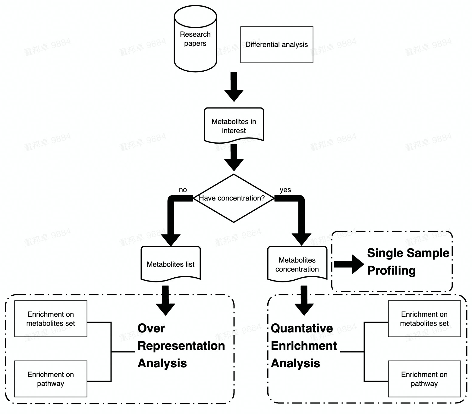
Following two chapters would focus on the Enrichment Analysis and Pathway Analysis of metabolomic data. Enrichment Analysis includes three sections (i.e., ORA, SSP and QEA) and Pathway Analysis only includes ORA and QEA.

The main difference between Enrichment Analysis and Pathway Analysis are the data set that input metabolites are enriched to. In Enrichment Analysis, input metabolites are enriched to pre-defined metabolite sets while in Pathway Analysis, metabolites are enriched to pathways in KEGG.

Workflow of Enrichment analysis and Pathway analysis is attached below. Users can choose analysis module according to their data type or interest.
Flowchart

See more details please go to the below tutorial (MetaboAnalyst website):

Functional Analysis Tutorial in MetaboAnalyst website

4.1 Enrichment Analysis

In this tutorial, we aim to help you to walk through the enrichment analysis in Metaboanalyst5.

This module performs metabolite set enrichment analysis (MSEA) for human and mammalian species based on several libraries containing ~9000 groups of metabolite sets. Users can upload either:

1) a list of compounds

2) a list of compounds with concentrations

3) a concentration table

Before carrying out the analysis, you are advised to acquire a list of metabolites in your interest (e.g., Statistical Analysis), then apply them to different modules in this tutorial according to the input file format.

Here, we apply SCFA sequencing data of stool samples in GvHD project as demo data.

4.1.1 Enviroment Setup

library(MetaboAnalystR)
library(tibble)
library(readxl)
library(magrittr)
#library(googledrive)

4.1.2 Over representation analysis (ORA)

ORA is used to evaluate whether a particular set of metabolites is represented more than expected by chance within a given compound list.
ORA is performed when the user provides only a list of compound names.

## Read input from the SCFA data of GvHD project.
SCFA_tbl <- readxl::read_xlsx('./dataset/InputFiles/GvHD_stool_metabolites_SCFA.xlsx') %>% 
  as.data.frame()

metabolite_lst <- SCFA_tbl$Compounds

## Create mSetObj, always initiate your mSet at the beginning.
mSet <- InitDataObjects("conc", "msetora", FALSE)

[1] “MetaboAnalyst R objects initialized …”

## Set up mSetObj with the list of compounds
mSet <- Setup.MapData(mSet, metabolite_lst)

## Cross reference list of compounds against libraries (hmdb, pubchem, chebi, kegg, metlin)
mSet <- CrossReferencing(mSet, "name")

[1] “Loaded files from MetaboAnalyst web-server.” [1] “Loaded files from MetaboAnalyst web-server.” [1] “1”
[2] “Name matching OK, please inspect (and manual correct) the results then proceed.”

## Example compound name map
mSet$name.map

$query.vec [1] “Acetic acid” “Propionic acid” “Isobutyric acid” “Butyric acid” “Isovaleric acid” “Valeric acid” “Hexanoic acid”

$hit.inx [1] 29 158 1241 28 566 708 409

$hit.values [1] “Acetic acid” “Propionic acid” “Isobutyric acid” “Butyric acid” “Isovaleric acid” “Valeric acid” “Caproic acid”

$match.state [1] 1 1 1 1 1 1 1

## Create the mapping results table
mSet <- CreateMappingResultTable(mSet)

[1] “Loaded files from MetaboAnalyst web-server.”

## Set the metabolite filter
mSet <- SetMetabolomeFilter(mSet, F)

## Select metabolite set library, we use fecal in this example, you can also choose "kegg_pathway", "smpdb_pathway", "blood", "urine", "csf", "snp", "predicted", "location", "drug, etc,.
mSet <- SetCurrentMsetLib(mSet, "fecal", 2)

## Calculate hypergeometric score, results table generated in your working directory
mSet <- CalculateHyperScore(mSet)

[1] “Loaded files from MetaboAnalyst web-server.”

ora_res <- read.csv('./msea_ora_result.csv', check.names = FALSE)
## Enrichment Ratio is computed by Hits / Expected, where hits = observed hits expected = expected hits (see the Table below)
knitr::kable(head(ora_res))

	total	expected	hits	Raw p	Holm p	FDR
Irritable Bowel Syndrome	93	0.5140	7	0e+00	4.0e-07	2.0e-07
Celiac Disease	98	0.5410	7	0e+00	6.0e-07	2.0e-07
Treated Celiac Disease	98	0.5410	7	0e+00	6.0e-07	2.0e-07
Juvenile Idiopathic Arthritis	3	0.0166	3	1e-07	4.1e-06	1.1e-06
Pervasive Developmental Disorder Not Otherwise Specified	82	0.4530	6	4e-07	1.6e-05	3.0e-06
Nonalcoholic Fatty Liver Disease	158	0.8730	7	4e-07	1.6e-05	3.0e-06

## Plot the ORA, bar-graph
mSet <- PlotORA(mSet, "./dataset/OutputFiles/ora_0_", "bar", "png", 250, width=NA)

knitr::include_graphics('./dataset/OutputFiles/ora_0_dpi250.png')

## Plot DotPlot
mSet <- PlotEnrichDotPlot(mSet, "ora", "./dataset/OutputFiles/ora_dot_0_", "png", 250, width=NA)

knitr::include_graphics('./dataset/OutputFiles/ora_dot_0_dpi250.png')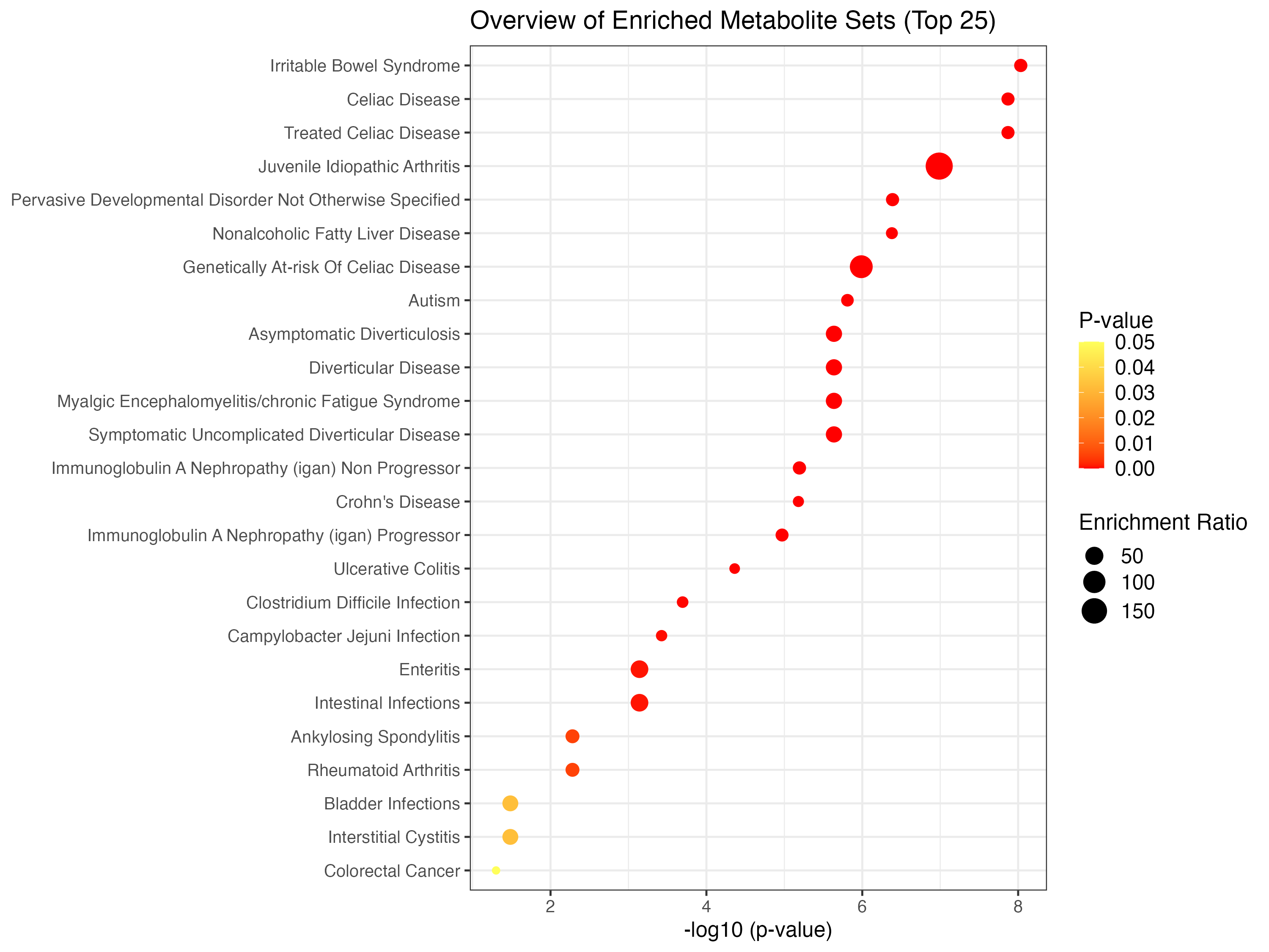

4.1.3 Clean environment 1

Remove all variables in env because a new mSet object needs to be created for the following analysis.

rm(list = ls())

4.1.4 Single Sample Profiling

For common human biofluids such as blood, urine, or CSF, normal concentration ranges are known for many metabolites.

In clinical metabolomic studies, it is often desirable to know whether certain metabolite concentrations in a given sample are significantly higher or lower than their normal ranges. MSEA’s SSP module is designed to provide this kind of analysis.

In particular, SSP is performed when the user provides a two-column list of both compounds and concentrations. When called, the SSP module will compare the measured concentration values of each compound to its recorded normal reference ranges of the corresponding biofluid.

Input for this module should be a list of metabolites and their concentrations (could be one column (1 x N) from a N * M abundance table with M samples/columns with N metabolites/rows).

## Read input from the SCFA data of GvHD project.
SCFA_tbl <- readxl::read_xlsx('./dataset/InputFiles/GvHD_stool_metabolites_SCFA.xlsx') %>% 
  as.data.frame()

## Initialize mSet object
mSet <- InitDataObjects("conc", "msetssp", FALSE)

[1] “MetaboAnalyst R objects initialized …”

## Read in metabolites names from SCFA_tbl
cmpd.vec <- SCFA_tbl$Compounds
mSet <- Setup.MapData(mSet, cmpd.vec)

## Read in concentration of sample CJY-V0 from SCFA_tbl
conc.vec <- SCFA_tbl$`CJY-V0`
mSet <- Setup.ConcData(mSet, conc.vec)

## Set unit of metabolites' concentration
mSet <- Setup.BiofluidType(mSet, "urine")

## Check names
mSet <- CrossReferencing(mSet, "name")

mSet <- CreateMappingResultTable(mSet)

[1] “Loaded files from MetaboAnalyst web-server.”

## Calculate SSP
mSet <- CalculateSSP(mSetObj = mSet)

[1] “Loaded files from MetaboAnalyst web-server.” [1] “Loaded files from MetaboAnalyst web-server.”

## Select all metabolites in our interests and do ORA.
mSet <- Setup.MapData(mSet, cmpd.vec)

## Filter
mSet <- SetMetabolomeFilter(mSet, F)

## Setup library
mSet <- SetCurrentMsetLib(mSet, "smpdb_pathway", 2)

## Calculate hyperscore
mSet <- CalculateHyperScore(mSet)

[1] “Loaded files from MetaboAnalyst web-server.”

ora_res <- read.csv('./msea_ora_result.csv',check.names = FALSE)

knitr::kable(head(ora_res))

	total	expected	hits	Raw p	Holm p	FDR
Fatty Acid Biosynthesis	35	0.2390	3	0.00117	0.114	0.114
Vitamin K Metabolism	14	0.0957	1	0.09210	1.000	1.000
Beta Oxidation of Very Long Chain Fatty Acids	17	0.1160	1	0.11100	1.000	1.000
Butyrate Metabolism	19	0.1300	1	0.12300	1.000	1.000
Ethanol Degradation	19	0.1300	1	0.12300	1.000	1.000
Mitochondrial Beta-Oxidation of Short Chain Saturated Fatty Acids	27	0.1850	1	0.17100	1.000	1.000

## Plot
mSet <- PlotORA(mSetObj = mSet, imgName = "./dataset/OutputFiles/SSP_ora_0_",
              imgOpt =  "net", format = "png", dpi = 250, width=NA)

knitr::include_graphics('./dataset/OutputFiles/SSP_ora_0_dpi250.png')

mSet <- PlotEnrichDotPlot(mSetObj = mSet, enrichType = "ora", 
                        imgName = "./dataset/OutputFiles/SSP_ora_dot_0_", 
                        format = "png", dpi = 250, width=NA)

knitr::include_graphics('./dataset/OutputFiles/SSP_ora_dot_0_dpi250.png')

4.1.5 Clean environment 2

Remove all variables in env because a new mSet object needs to be created for the following analysis.

rm(list = ls())

4.1.6 Quantitative Enrichment Analysis (QEA)

QEA is performed when the user uploads a concentration table containing metabolite concentration data from multiple samples.

QEA is based on the globaltest algorithm to perform enrichment analysis directly from raw concentration data and does not require a list of significantly changed compounds.

Especially, QEA adopted globaltest as the backend. Please find citation for detailed introduction.
In short, globaltest calculates Q values, the formula to calculate Q-statistic can be obtained from the original publication by (Goeman JJ, et al). Q-statistic can be intuitively interpreted as an aggregate of squared covariance between concentration changes and the phenotypes - compounds with large variance have much more influence on the Q than compound with small variance.

And the null hypothesis in QEA to be tested are made to be whether two groups of samples are not different with respect to their overall metabolites’ abundance pattern. Under this hypothesis, expectation and standard deviation can be calculated and p value can be estimated. If p < 0.05, it means that two groups of samples are different with respect to their overall metabolites’ abundance pattern.

## Create mSetObj
mSet <- InitDataObjects("conc", "msetqea", FALSE)

Starting Rserve: /Library/Frameworks/R.framework/Resources/bin/R CMD /Library/Frameworks/R.framework/Versions/4.1/Resources/library/Rserve/libs//Rserve –no-save

[1] “MetaboAnalyst R objects initialized …”

## Read in data table
SCFA_tbl <- readxl::read_xlsx('./dataset/InputFiles/GvHD_stool_metabolites_SCFA.xlsx') %>% 
  as.data.frame()

## Replace N/A with NA
SCFA_tbl[SCFA_tbl == "N/A"] <- NA

## Select columns from input data table
SCFA_tbl <- SCFA_tbl[,c(2,5:ncol(SCFA_tbl))] %>% column_to_rownames('Compounds') %>% 
  t() %>% as.data.frame()

## Create Group Info
SCFA_tbl %<>% dplyr::mutate(Group = c(rep('A',25), rep('B',31))) %>% 
  dplyr::select(c('Group', colnames(.)[colnames(.) != 'Group'])) %>% 
  rownames_to_column('Samples')

## Write data table in csv file
write.csv(SCFA_tbl, './dataset/OutputFiles/GvHD_stool_metabolites_SCFA.csv', row.names = FALSE)

## Read in data table
mSet <- Read.TextData(mSet, "./dataset/OutputFiles/GvHD_stool_metabolites_SCFA.csv", "rowu", "disc")

# Perform cross-referencing of compound names
mSet <- CrossReferencing(mSet, "name")

# Create mapping results table
mSet <- CreateMappingResultTable(mSet)

[1] “Loaded files from MetaboAnalyst web-server.”

# Mandatory check of data
mSet <- SanityCheckData(mSet)

[1] “Successfully passed sanity check!”
[2] “Samples are not paired.”
[3] “2 groups were detected in samples.”
[4] “Only English letters, numbers, underscore, hyphen and forward slash (/) are allowed.”
[5] “Other special characters or punctuations (if any) will be stripped off.”
[6] “All data values are numeric.”
[7] “A total of 26 (6.6%) missing values were detected.”
[8] “By default, missing values will be replaced by 1/5 of min positive values of their corresponding variables” [9] “Click the Proceed button if you accept the default practice;”
[10] “Or click the Missing Values button to use other methods.”

# Replace missing values with minimum concentration levels
mSet <- ReplaceMin(mSet)

# Perform no normalization
mSet <- PreparePrenormData(mSet)

#mSet <- Normalization(mSet, rowNorm = "SumNorm", transNorm = "LogNorm", scaleNorm = "ParetoNorm", ref = "PIF_178", ratio=FALSE, ratioNum=20)
mSet <- Normalization(mSet, rowNorm = "SumNorm", transNorm = "LogNorm", scaleNorm = "ParetoNorm")

# Plot normalization
mSet <- PlotNormSummary(mSet, "./dataset/OutputFiles/norm_0_", "png", 250, width=NA)

knitr::include_graphics('./dataset/OutputFiles/norm_0_dpi250.png')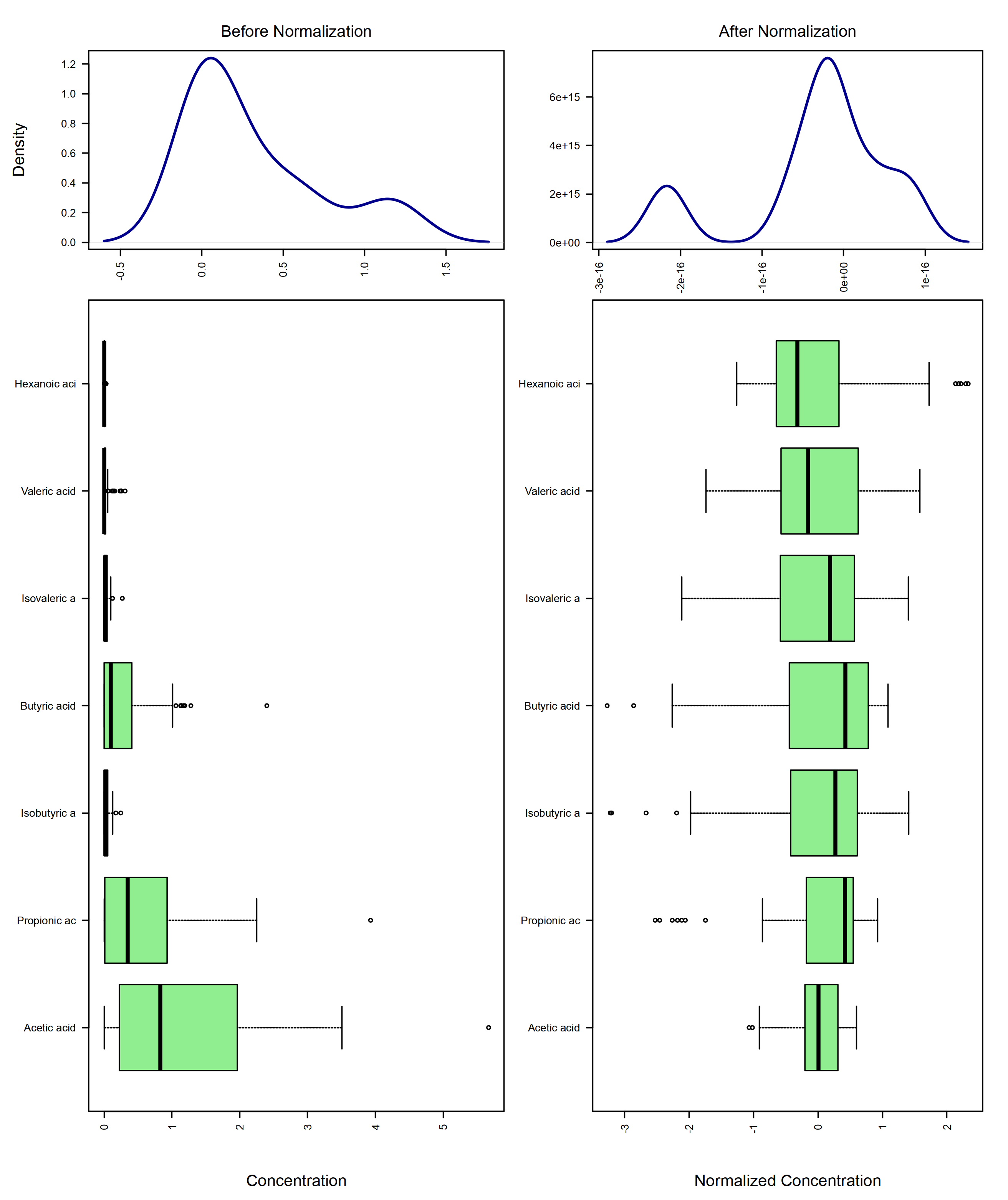

# Plot sample-wise normalization
mSet <- PlotSampleNormSummary(mSet, "./dataset/OutputFiles/snorm_0_", "png", 250, width=NA)

knitr::include_graphics('./dataset/OutputFiles/snorm_0_dpi250.png')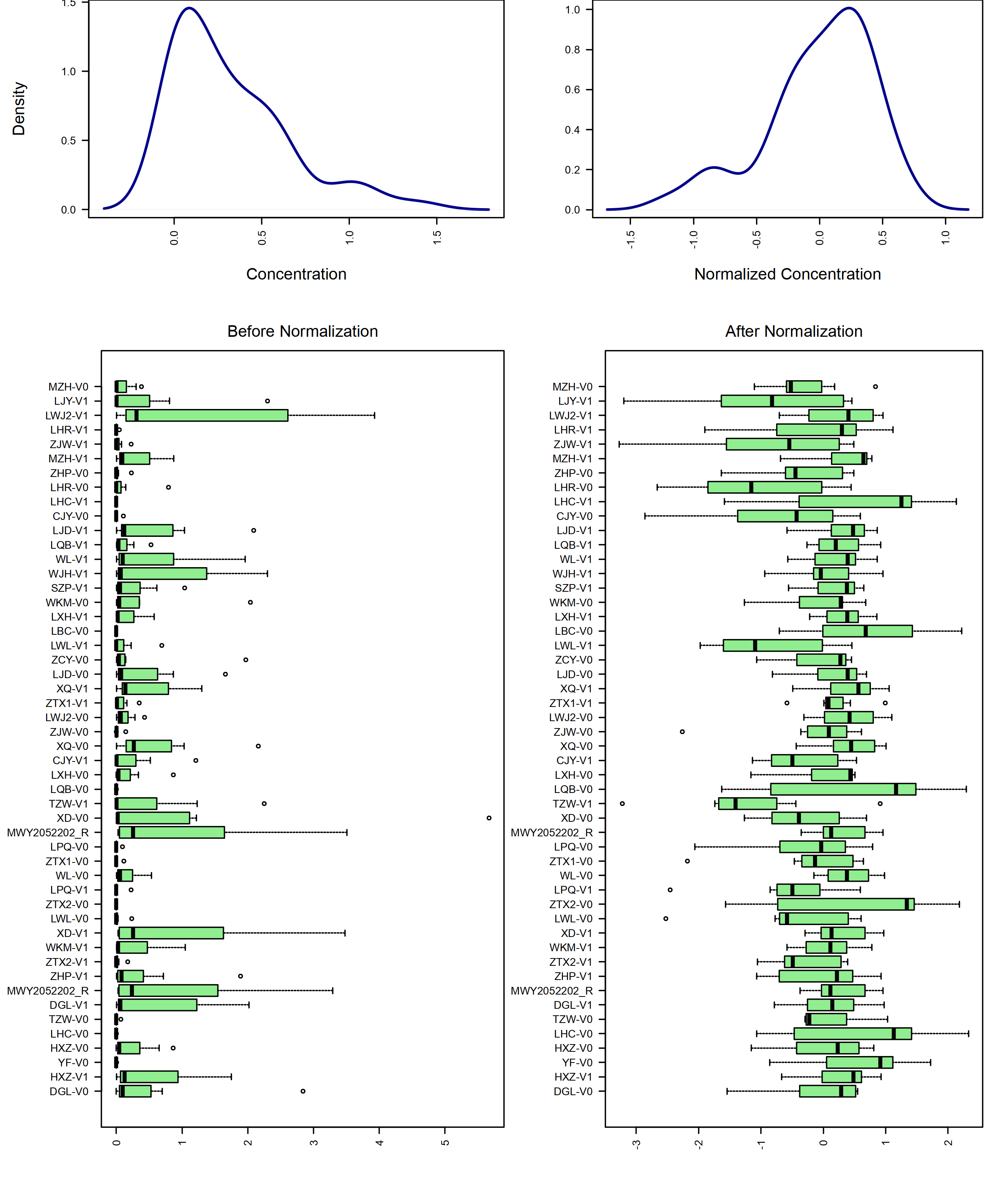

# Set the metabolome filter
mSet <- SetMetabolomeFilter(mSet, F)

# Set the metabolite set library to pathway
mSet <- SetCurrentMsetLib(mSet, "smpdb_pathway", 2)

# Calculate the global test score
mSet <- CalculateGlobalTestScore(mSet)

[1] “Loaded files from MetaboAnalyst web-server.”

msea_qea_res <- read.csv('./msea_qea_result.csv')

knitr::kable(head(msea_qea_res))

X	Total.Cmpd	Hits	Statistic.Q	Expected.Q	Raw.p	Holm.p	FDR
Propanoate Metabolism	42	1	4.3168	1.8182	0.12440	1	0.62002
Vitamin K Metabolism	14	1	4.3168	1.8182	0.12440	1	0.62002
Butyrate Metabolism	19	1	2.1853	1.8182	0.27692	1	0.62002
Fatty Acid Biosynthesis	35	3	1.7437	1.8182	0.37316	1	0.62002
Beta Oxidation of Very Long Chain Fatty Acids	17	1	1.4123	1.8182	0.38302	1	0.62002
Mitochondrial Beta-Oxidation of Short Chain Saturated Fatty Acids	27	1	1.4123	1.8182	0.38302	1	0.62002

# Plot the QEA
mSet <- PlotQEA.Overview(mSet, "./dataset/OutputFiles/qea_0_", "bar", "png", 250, width=NA)

knitr::include_graphics('./dataset/OutputFiles/qea_0_dpi250.png')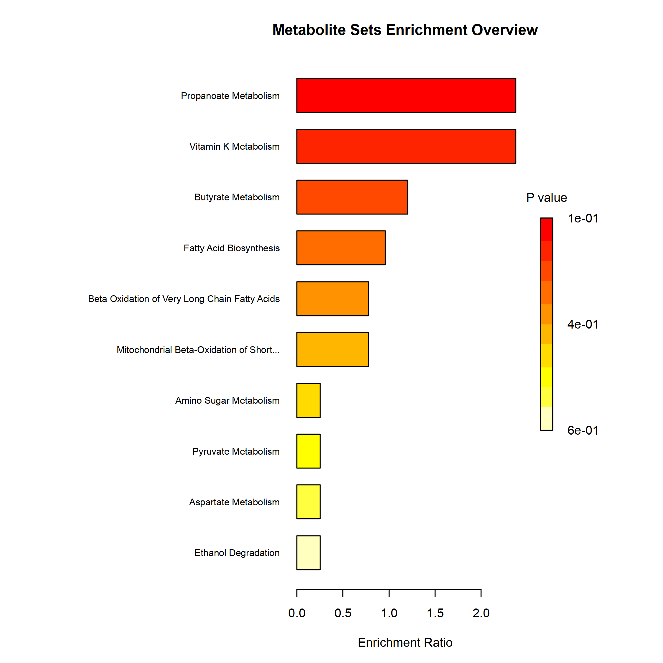

mSet <- PlotEnrichDotPlot(mSet, "qea", "./dataset/OutputFiles/qea_dot_0_", "png", 250, width=NA)

knitr::include_graphics('./dataset/OutputFiles/qea_dot_0_dpi250.png')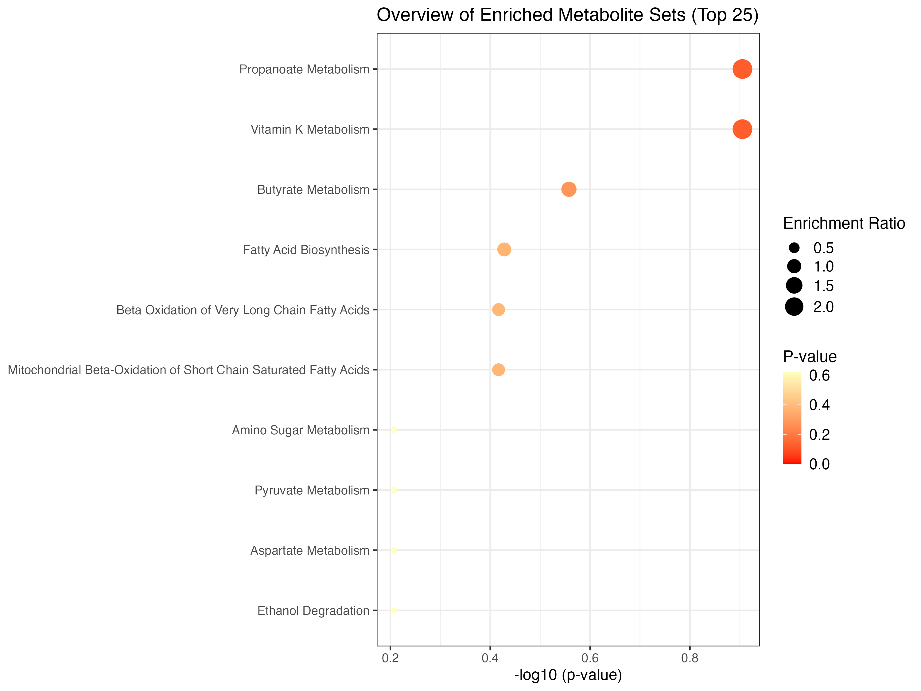

Remove all variables in env because a new mSet object needs to be created for the following analysis.

rm(list = ls())

4.2 Pathway Analysis

In this tutorial, we aim to help you to walk through the pathway analysis in Metaboanalyst5.

This module supports pathway analysis (integrating enrichment analysis and pathway topology analysis) and visualization for 26 model organisms, including Human, Mouse, Rat, Cow, Chicken, Zebrafish, Arabidopsis thaliana, Rice, Drosophila, Malaria, S. cerevisae, E.coli, and others species.

Here, we apply TM metabolites sequencing data of stool samples in GvHD project as demo data. Moreover, to reduce data noise, we selected differentially abundant metabolites in aGVHD patients from the differential analysis result in Xu XiaoMin’s analysis.

4.2.1 Enviroment Set up

4.2.2 Over representation analysis

Similar to ORA in Enrichment analysis.

## Read in differentially abundant TM metanolites data from GVHD project
DA_metabolites <- readxl::read_xlsx('./dataset/InputFiles/DA_metabolites_agvhd_adult_result.xlsx') %>% 
  as.data.frame()

## Create vector consisting of compounds for enrichment analysis
tmp.vec <- DA_metabolites$Compounds

## Create mSetObj for storing objects created during your analysis
mSet <- InitDataObjects("conc", "pathora", FALSE)

[1] “MetaboAnalyst R objects initialized …”

## Set up mSetObj with the list of compounds
mSet <- Setup.MapData(mSet, tmp.vec)

## Cross reference list of compounds against libraries (hmdb, pubchem, chebi, kegg, metlin). This step is to make sure that all metabolites names provided match the metabolites' names in KEGG database.
mSet <- CrossReferencing(mSet, "name")

[1] “Loaded files from MetaboAnalyst web-server.” [1] “Loaded files from MetaboAnalyst web-server.” [1] “0”
[2] “Over half of the compound IDs could not be matched to our database. Please make sure that correct compound IDs or common compound names are used.”

## Remove metabolites failed to match the metabolites' names in KEGG database.
tmp.vec <- tmp.vec[mSet$name.map$match.state == 1]

## Re-initialize mSet object
mSet <- InitDataObjects("conc", "pathora", FALSE)

## Set up mSetObj with the matched list of compounds
mSet <- Setup.MapData(mSet, tmp.vec)

## Cross reference list of compounds against libraries (hmdb, pubchem, chebi, kegg, metlin). Check again if all metabolites' names have their matches in KEGG database
mSet <- CrossReferencing(mSet, "name")

## Creates a mapping result table shows HMDB, KEGG, PubChem, etc. IDs. Saved as "name_map.csv" or can be found in mSet$dataSet$map.table. Compounds with no hits will contain NAs across the columns.
mSet <- CreateMappingResultTable(mSet)

[1] “Loaded files from MetaboAnalyst web-server.”

## Select the pathway library, ranging from mammals to prokaryotes
## Note the third parameter, where users need to input the KEGG pathway version.
## Use "current" for the latest KEGG pathway library or "v2018" for the KEGG pathway library version prior to November 2019.
mSet <- SetKEGG.PathLib(mSet, "hsa", "current")

## Set the metabolite filter. Default set to false
mSet <- SetMetabolomeFilter(mSet, F)

## Calculate the over representation analysis score, here we selected to use the hypergeometric test (alternative is Fisher's exact test)
## A results table "pathway_results.csv" will be created and found within your working directory
# mSet <- CalculateOraScore(mSet, "rbc", "hyperg")
# 
# pathway_res <- read.csv('./pathway_results.csv')
# 
# knitr::kable(head(pathway_res))
# 
# # Plot of the Pathway Analysis Overview
# mSet <- PlotPathSummary(mSet,show.grid=FALSE, "./dataset/OutputFiles/path_view_0_", "png", dpi =250, width=NA)

knitr::include_graphics('./dataset/OutputFiles/path_view_0_dpi250.png')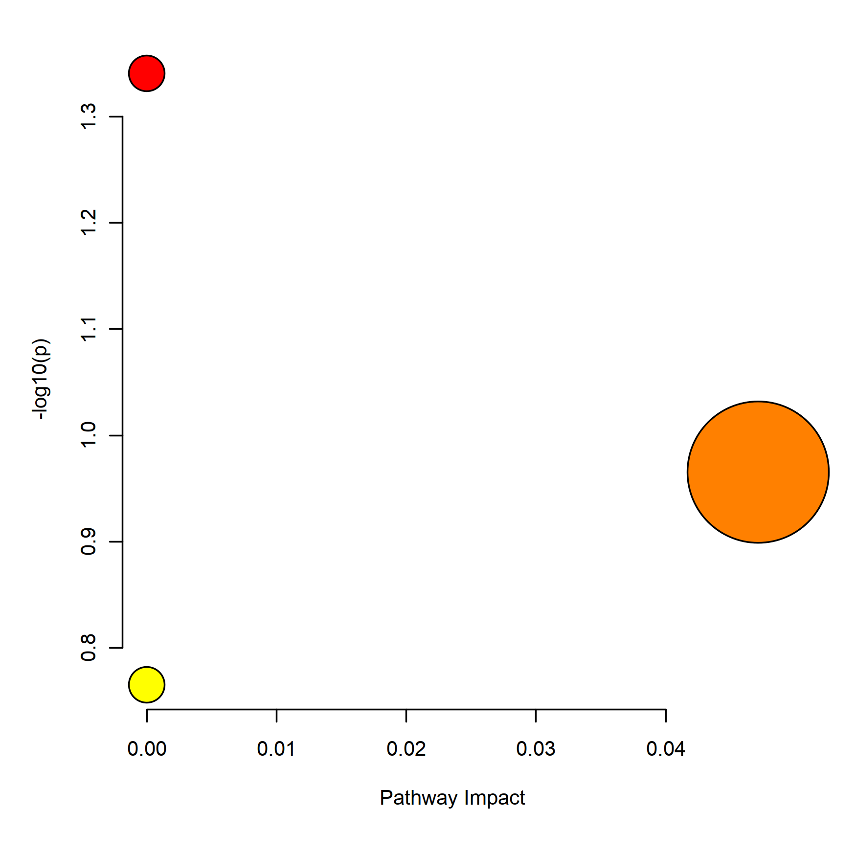

# Plot a specific metabolic pathway, in this case "Glycine, serine and threonine metabolism"
# mSet <- PlotKEGGPath(mSetObj = mSet, pathName = "Glycine, serine and threonine metabolism", 528, 480, "png", dpi=72)

4.2.3 Clean environment 3

rm(list = ls())

4.2.4 Concentration Table (QEA)

Similar to QEA in Enrichment analysis.

KO enrichment is calculated via the global test algorithm when abundance of metabolites are provided.

Global test evaluates whether a set of genes (i.e. KEGG pathways) is significantly associated with a variable of interest. Compared to ORA, which uses only the total number of KO hits in a pathway, global test considers the gene abundance values and is considered to be more sensitive than ORA. It assumes that if a gene set can be used to predict an outcome of interest, the gene expression patterns per outcome must be different.

The global test algorithm is implemented in MicrobiomeAnalyst using the globaltest R package. P-values for both methods are corrected for multiple-testing using the Benjamini and Hochberg’s False-Discovery Rate (FDR).

In this module, we use differentially abundant metabolites in aGVHD patients from the differential analysis result in Xu XiaoMin’s analysis and their abundance as input.

## Read in differentially abundant TM metanolites data from GVHD project
DA_metabolites <- readxl::read_xlsx('./dataset/InputFiles/DA_metabolites_agvhd_adult_result.xlsx') %>% 
  as.data.frame()

## Initialize data object
mSet <- InitDataObjects("conc", "pathqea", FALSE)

Starting Rserve: /Library/Frameworks/R.framework/Resources/bin/R CMD /Library/Frameworks/R.framework/Versions/4.1/Resources/library/Rserve/libs//Rserve –no-save

[1] “MetaboAnalyst R objects initialized …”

## Read in data table
input_df <- readxl::read_xlsx('./dataset/InputFiles/GvHD_stool_metabolites_TM.xlsx') %>% 
  as.data.frame() %>% 
  .[,c(2,25:ncol(.))] %>% 
  column_to_rownames('Compounds') %>% 
  .[DA_metabolites$Compounds,] %>% 
  t() %>% 
  as.data.frame()

Groupinfo <- rownames(input_df) %>% 
  stringr::str_split('-') %>% 
  as.data.frame() %>% 
  .[2,] %>% 
  unlist() %>% 
  as.vector()

input_df %<>% dplyr::mutate(Group = Groupinfo) %>% 
  dplyr::select(c('Group', colnames(.)[colnames(.) != 'Group'])) %>% 
  rownames_to_column('Sample')

## Write reformed metabolites abundance table into csv file
write.csv(input_df, './dataset/OutputFiles/GvHD_stool_metabolites_TM.csv',row.names = FALSE)

mSet <- Read.TextData(mSet, './dataset/OutputFiles/GvHD_stool_metabolites_TM.csv', "rowu", "disc")

## Show first few rows in data table
knitr::kable(head(input_df))

Sample	Group	Erucic acid	5-Methylcytosine	D-Gluconic Acid	LPE(14:0/0:0)	N-Acetylglucosamine 1-Phosphate	7-ketodeoxycholic acid	Bis(1-inositol) -3,1’-phosphate 1-phosphate	Asp-phe	Phenylacetyl-L-Glutamine	N-Acetylglycine	Carnitine C2:0	Acetylcholine	Lithocholic acid	3-Carboxypropyltrimethylammonium	Biotinamide	5’-deoxy-5’-fluoroadenosine	Carnitine C5:1	Val-Val	Gly Leu Tyr	Ile-Thr	Isoleucyl-Serine	Isoleucyl-Tyrosine	Phe Val Ala	Phosphonic acid, P-[(3R)-3-amino-4-[(3-hexylphenyl)amino]-4-oxobutyl]-	2-[2,4-dihydroxy-3-(3-methylbut-2-en-1-yl)phenyl]-1-[2,4,6-trihydroxy-3-(3-methylbut-2-en-1-yl)phenyl]propan-1-one	Asp Ile Ile	Gly Leu Val	Ile Glu Leu	Ile Ile Asn	Lys Pro Ile	Phylloquinone oxide	Thr Val Met	Val Leu Thr	(2R,3S,4R,5R)-2,3,4,5,6-pentahydroxyhexanoate
TZW-V0	V0	1629500	630750	11598000	1900000	1048900	142580.0	4516900	1896000	483960	75306000	35820000	169220	30462	169220	72050	52622	48756	6690500	382840	151620	863010	3696700	371890	419900	376300	1992200	304420	321110	243390	17617	3885	1950000	582200	208490000
LBC-V0	V0	17057	220290	8239500	68958	9880900	6446.1	313960	19488000	569570	11310000	81713000	90812	9	90812	533990	9	338900	1044600	9	99102	468170	7789300	46193	88988	14154	463070	10903	32430	29187	12902000	9	333220	210680	166450000
HXZ-V0	V0	3719000	316360	91189	14390000	37784000	21965000.0	459320	5671200	8502200	6758300	71495000	518950	438800	518950	1222000	36295	953350	8538900	88531	454250	952750	56697	45953	115110	2798900	348560	79613	134400	438750	7569200	24432	747830	86317	2163600
LJY-V0	V0	1641600	285270	72194	7366800	9557700	3289400.0	71782	756830	30602	531930	387590	1345400	6488400	1345400	544550	27188	295820	3163500	136380	180510	819430	21168	171330	159850	1478200	804870	128420	910850	379890	78433	459240	576110	123100	1502600
CJY-V0	V0	9	45013	25589	882500	561320	1603.1	9	7463500	556470	5814900	13723000	26319	9	26319	182350	18175	135980	1555700	38015	130400	441760	3275600	235320	154660	169880	568150	35916	48067	215340	328930	9	763870	97575	900440
WKM-V0	V0	3079600	228130	396980	8410000	12296000	7266400.0	42405	13785000	4553400	9620400	1311800	4392400	9	4392400	74831	79472	48558	5309200	88741	221440	593130	44678	250550	140720	1660200	522490	234090	263740	415690	9312900	586940	619550	136990	8894600

## Check metabolites Names of input table. Found >15 compounds without matches.
mSet <- CrossReferencing(mSet, "name")

## Keep matched metabolites
metabolites_keep <- mSet$name.map$query.vec[mSet$name.map$match.state == 1]
input_df <- input_df[c('Sample','Group', metabolites_keep)]

## Overwrite previously generated abundance csv file with matched metabolites
write.csv(input_df, './dataset/OutputFiles/GvHD_stool_metabolites_TM.csv',row.names = FALSE)

## Initialize data object again
mSet <- InitDataObjects("conc", "pathqea", FALSE)

## Read in updated metabolites abundance table
mSet <- Read.TextData(mSet, './dataset/OutputFiles/GvHD_stool_metabolites_TM.csv', "rowu", "disc")

## Check Sanity and replace 0
mSet <- SanityCheckData(mSet)

[1] “Successfully passed sanity check!”
[2] “Samples are not paired.”
[3] “2 groups were detected in samples.”
[4] “Only English letters, numbers, underscore, hyphen and forward slash (/) are allowed.”
[5] “Other special characters or punctuations (if any) will be stripped off.”
[6] “All data values are numeric.”
[7] “A total of 0 (0%) missing values were detected.”
[8] “By default, missing values will be replaced by 1/5 of min positive values of their corresponding variables” [9] “Click the Proceed button if you accept the default practice;”
[10] “Or click the Missing Values button to use other methods.”

mSet <- ReplaceMin(mSet)

## Check metabolites Names of input table again
mSet <- CrossReferencing(mSet, "name")

## Creates a mapping result table shows HMDB, KEGG, PubChem, etc. IDs. Saved as "name_map.csv" or can be found in mSet$dataSet$map.table. Compounds with no hits will contain NAs across the columns.
mSet <- CreateMappingResultTable(mSet)

[1] “Loaded files from MetaboAnalyst web-server.”

## Normalize
mSet <- PreparePrenormData(mSet)
mSet <- Normalization(mSet, rowNorm = "SumNorm", transNorm = "LogNorm", scaleNorm = "ParetoNorm")
mSet <- PlotNormSummary(mSet, 
                        imgName = "./dataset/OutputFiles/kegg_pathnorm_0_", 
                        format = "png", dpi = 250, width=NA)

knitr::include_graphics('./dataset/OutputFiles/kegg_pathnorm_0_dpi250.png')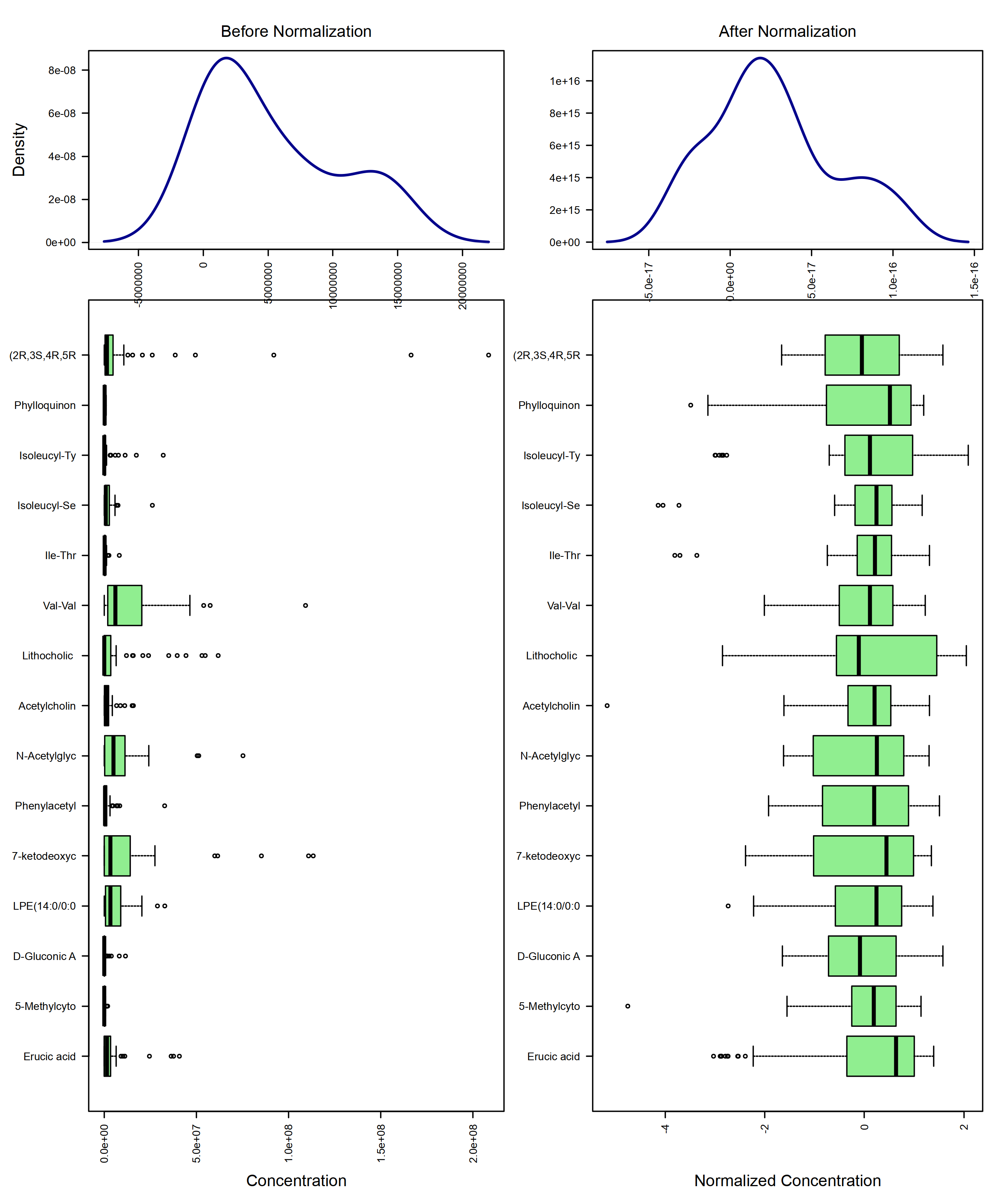

mSet <- PlotSampleNormSummary(mSet, "./dataset/OutputFiles/kegg_pathsnorm_0_", "png", 250, width=NA)

knitr::include_graphics('./dataset/OutputFiles/kegg_pathsnorm_0_dpi250.png')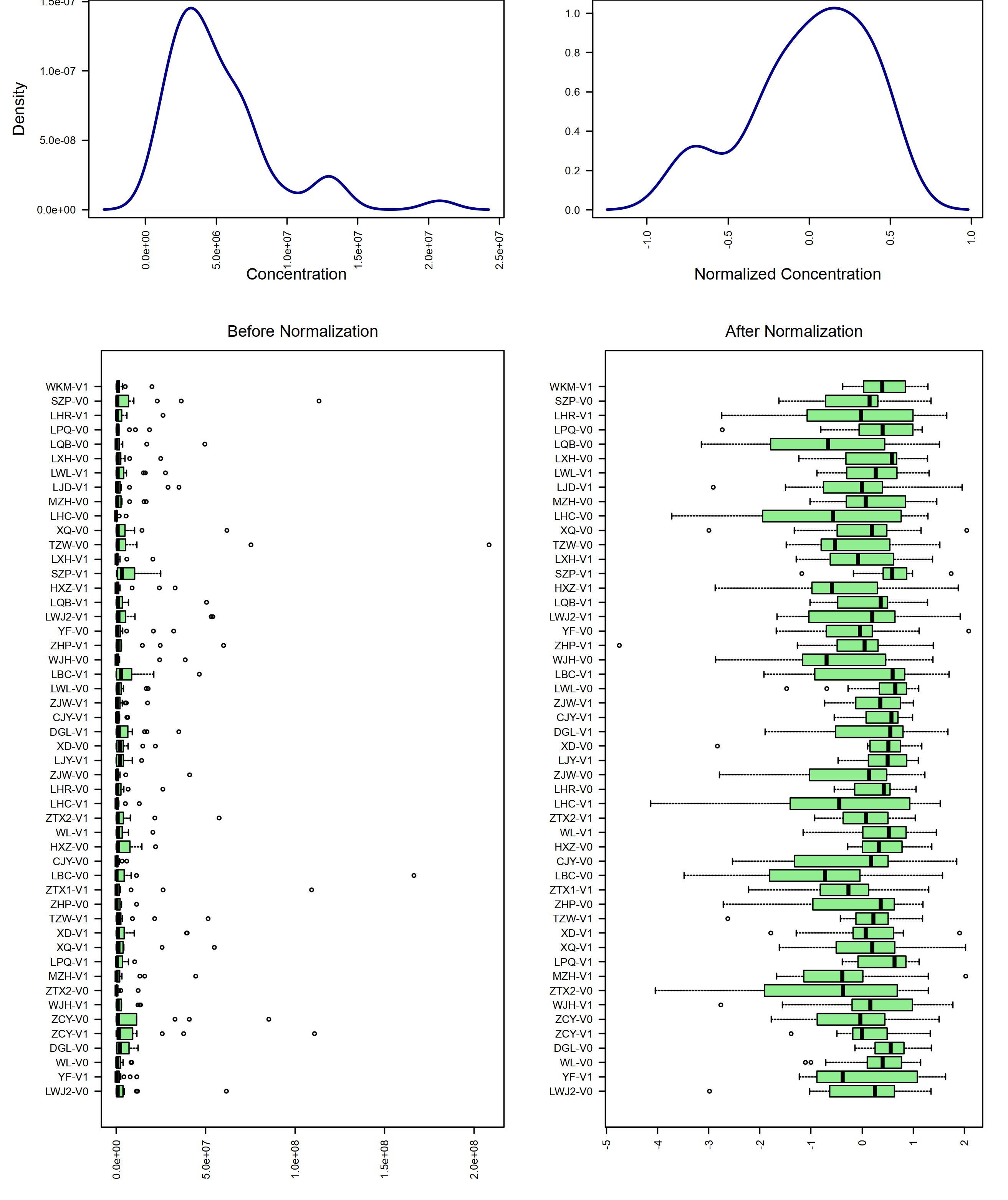

## Enrich to KEGG
mSet <- SetKEGG.PathLib(mSet, "hsa", "current")
mSet <- SetMetabolomeFilter(mSet, F)
mSet <- CalculateQeaScore(mSet, "rbc", "gt")

[1] “Loaded files from MetaboAnalyst web-server.” [1] “http://api.xialab.ca/pathwayqea” [1] “Failed to connect to Xia Lab API Server!”

# pathway_res <- read.csv('./pathway_results.csv', check.names = FALSE)

# knitr::kable(head(pathway_res))

# mSet <- PlotPathSummary(mSet, F, "./dataset/OutputFiles/kegg_path_view_0_", "png", 250, width=NA, NA, NA )

knitr::include_graphics('./dataset/OutputFiles/kegg_path_view_0_dpi250.png')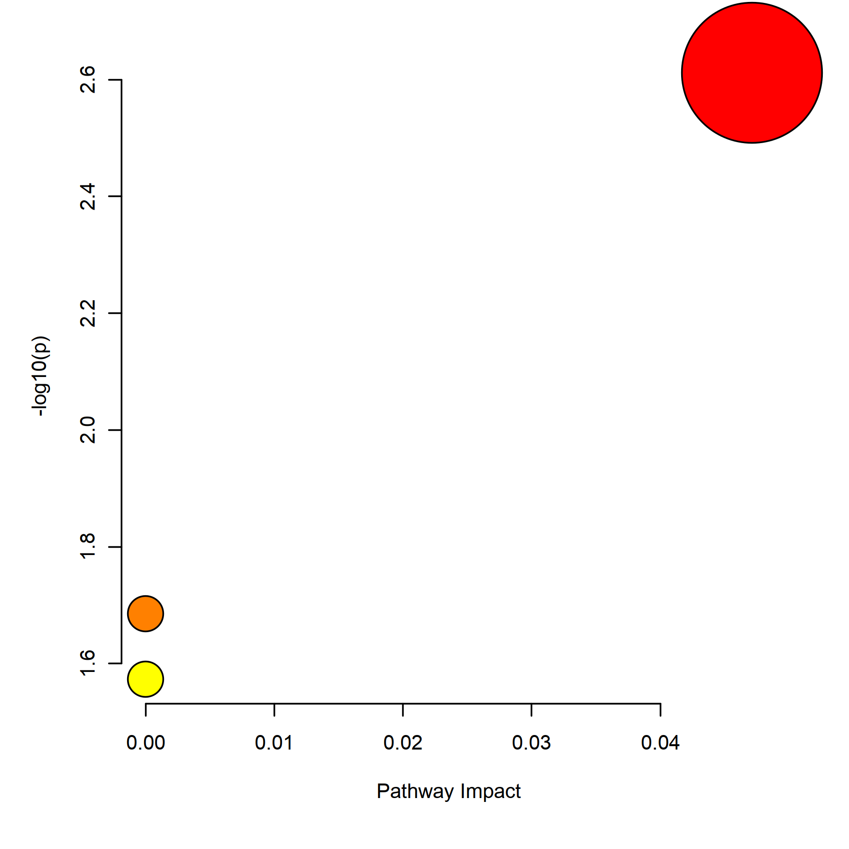

## Plot specified pathway map
# mSet <- PlotKEGGPath(mSet, "Phenylalanine, tyrosine and tryptophan biosynthesis",576, 480, "png", NULL)
# mSet <- RerenderMetPAGraph(mSet, "zoom1658398230135.png",576.0, 480.0, 100.0)
# mSet <- PlotKEGGPath(mSet, "Glycine, serine and threonine metabolism",576, 480, "png", NULL)

4.3 Functional Analysis by R package

Functional Analysis for DE metabolites
- ORA: Over Representive Analysis
- GSEA: Gene Set Enrichment Analysis

4.3.1 Loading R packages

library(dplyr)
library(tibble)
library(ggplot2)
library(clusterProfiler)
library(org.Mm.eg.db)
library(readxl)
library(ropls)
library(Biobase)
library(SummarizedExperiment)

library(massdatabase)
library(MicrobiomeProfiler)

4.3.2 Importing Data

ExprSet <- readRDS("./dataset/POMA/ExprSet_raw.RDS")
se_impute <- readRDS("./dataset/POMA/se_impute.RDS")
se_norm <- readRDS("./dataset/POMA/se_normalize.RDS")

4.3.3 Differential Analysis

Fold change (group1 vs group2)
- RawData
VIP (Variable influence on projection & coefficient)
- Variable influence on projection (VIP) for orthogonal projections to latent structures (OPLS)
- Variable influence on projection (VIP) for projections to latent structures (PLS)
T-test
- significant differences between two groups (p value)
Merging result
- Foldchange by Raw Data
- VIP by Normalized Data
- test Pvalue by Normalized Data

FoldChange <- function(
    x,
    group,
    group_names) {
  
  # dataseat
  metadata <- SummarizedExperiment::colData(x) %>%
      as.data.frame()
  profile <- SummarizedExperiment::assay(x) %>%
      as.data.frame()

  colnames(metadata)[which(colnames(metadata) == group)] <- "CompVar"
  phenotype <- metadata %>%
    dplyr::filter(CompVar %in% group_names) %>%
    dplyr::mutate(CompVar = as.character(CompVar)) %>%
    dplyr::mutate(CompVar = factor(CompVar, levels = group_names))
  
  sid <- intersect(rownames(phenotype), colnames(profile))
  phen <- phenotype[pmatch(sid, rownames(phenotype)), , ]
  prof <- profile %>%
    dplyr::select(all_of(sid))
  
  if (!all(colnames(prof) == rownames(phen))) {
    stop("Wrong Order")
  }
  
  fc_res <- apply(prof, 1, function(x1, y1) {
    dat <- data.frame(value = as.numeric(x1), group = y1)
    mn <- tapply(dat$value, dat$group, function(x){
      mean(x, na.rm = TRUE)
    }) %>%
      as.data.frame() %>% 
      stats::setNames("value") %>%
      tibble::rownames_to_column("Group")

    mn1 <- with(mn, mn[Group %in% group_names[1], "value"])
    mn2 <- with(mn, mn[Group %in% group_names[2], "value"])
    mnall <- mean(dat$value, na.rm = TRUE)
    
    if (all(mn1 != 0, mn2 != 0)) {
      fc <- mn1 / mn2
    } else {
      fc <- NA
    }
    
    logfc <- log2(fc)

    res <- c(fc, logfc, mnall, mn1, mn2)
    return(res)
  }, phen$CompVar) %>%
    base::t() %>% data.frame() %>%
    tibble::rownames_to_column("Feature")
  
  colnames(fc_res) <- c("FeatureID", "FoldChange", 
                        "Log2FoldChange",
                        "Mean Abundance\n(All)",
                     paste0("Mean Abundance\n", c("former", "latter")))  
  
  # Number of Group
  dat_status <- table(phen$CompVar)
  dat_status_number <- as.numeric(dat_status)
  dat_status_name <- names(dat_status)
  fc_res$Block <- paste(paste(dat_status_number[1], dat_status_name[1], sep = "_"),
                       "vs",
                       paste(dat_status_number[2], dat_status_name[2], sep = "_"))
  
  res <- fc_res %>%
      dplyr::select(FeatureID, Block, everything())    

  return(res)
}

VIP_fun <- function(
    x,
    group,
    group_names,
    VIPtype = c("OPLS", "PLS"),
    vip_cutoff = 1) {
  
  metadata <- SummarizedExperiment::colData(x) %>%
      as.data.frame()
  profile <- SummarizedExperiment::assay(x) %>%
      as.data.frame()

  colnames(metadata)[which(colnames(metadata) == group)] <- "CompVar"
  phenotype <- metadata %>%
    dplyr::filter(CompVar %in% group_names) %>%
    dplyr::mutate(CompVar = as.character(CompVar)) %>%
    dplyr::mutate(CompVar = factor(CompVar, levels = group_names))
  
  sid <- intersect(rownames(phenotype), colnames(profile))
  phen <- phenotype[pmatch(sid, rownames(phenotype)), , ]
  prof <- profile %>%
    dplyr::select(all_of(sid))
  
  if (!all(colnames(prof) == rownames(phen))) {
    stop("Wrong Order")
  }
  
  dataMatrix <- prof %>% base::t() # row->sampleID; col->features
  sampleMetadata <- phen # row->sampleID; col->features
  
  comparsionVn <- sampleMetadata[, "CompVar"]
  
  # corrlation between group and features
  pvaVn <- apply(dataMatrix, 2,
                 function(feaVn) cor.test(as.numeric(comparsionVn), feaVn)[["p.value"]])
  
  if (VIPtype == "OPLS") {
    vipVn <- getVipVn(opls(dataMatrix, 
                           comparsionVn,
                           predI = 1, 
                           orthoI = NA,
                           fig.pdfC = "none"))    
  } else {
    vipVn <- getVipVn(opls(dataMatrix, 
                           comparsionVn,
                           predI = 1, 
                           fig.pdfC = "none"))    
  }
  quantVn <- qnorm(1 - pvaVn / 2)
  rmsQuantN <- sqrt(mean(quantVn^2))
  
  opar <- par(font = 2, font.axis = 2, font.lab = 2,
              las = 1,
              mar = c(5.1, 4.6, 4.1, 2.1),
              lwd = 2, pch = 16)
  plot(pvaVn, 
       vipVn,
       col = "red",
       pch = 16,
       xlab = "p-value", ylab = "VIP", xaxs = "i", yaxs = "i")
  box(lwd = 2)
  curve(qnorm(1 - x / 2) / rmsQuantN, 0, 1, add = TRUE, col = "red", lwd = 3)
  abline(h = 1, col = "blue")
  abline(v = 0.05, col = "blue")
  
  res_temp <- data.frame(
      FeatureID = names(vipVn),
      VIP = vipVn,
      CorPvalue = pvaVn) %>%
    dplyr::arrange(desc(VIP))

  vip_select <- res_temp %>%
    dplyr::filter(VIP > vip_cutoff) 
  
  pl <- ggplot(vip_select, aes(FeatureID, VIP)) +
    geom_segment(aes(x = FeatureID, xend = FeatureID,
                     y = 0, yend = VIP)) +
    geom_point(shape = 21, size = 5, color = '#008000' ,fill = '#008000') +
    geom_point(aes(1,2.5), color = 'white') +
    geom_hline(yintercept = 1, linetype = 'dashed') +
    scale_y_continuous(expand = c(0, 0)) +
    labs(x = '', y = 'VIP value') +
    theme_bw() +
    theme(legend.position = 'none',
          legend.text = element_text(color = 'black',size = 12, family = 'Arial', face = 'plain'),
          panel.background = element_blank(),
          panel.grid = element_blank(),
          axis.text = element_text(color = 'black',size = 15, family = 'Arial', face = 'plain'),
          axis.text.x = element_text(angle = 90),
          axis.title = element_text(color = 'black',size = 15, family = 'Arial', face = 'plain'),
          axis.ticks = element_line(color = 'black'),
          axis.ticks.x = element_blank())
  
  # Number of Group
  dat_status <- table(phen$CompVar)
  dat_status_number <- as.numeric(dat_status)
  dat_status_name <- names(dat_status)
  res_temp$Block <- paste(paste(dat_status_number[1], dat_status_name[1], sep = "_"),
                       "vs",
                       paste(dat_status_number[2], dat_status_name[2], sep = "_"))

  res_df <- res_temp %>%
      dplyr::select(FeatureID, Block, everything())    


  res <- list(vip = res_df,
              plot = pl)
  
  return(res)
}

t_fun <- function(
    x,
    group,
    group_names) {
  
  # dataseat
  metadata <- SummarizedExperiment::colData(x) %>%
      as.data.frame()
  profile <- SummarizedExperiment::assay(x) %>%
      as.data.frame()

  # rename variables
  colnames(metadata)[which(colnames(metadata) == group)] <- "CompVar" 
  
  phenotype <- metadata %>%
    dplyr::filter(CompVar %in% group_names) %>%
    dplyr::mutate(CompVar = as.character(CompVar)) %>%
    dplyr::mutate(CompVar = factor(CompVar, levels = group_names))
  
  sid <- intersect(rownames(phenotype), colnames(profile))
  phen <- phenotype[pmatch(sid, rownames(phenotype)), , ]
  prof <- profile %>%
    dplyr::select(all_of(sid))
  
  if (!all(colnames(prof) == rownames(phen))) {
    stop("Wrong Order")
  }

  t_res <- apply(prof, 1, function(x1, y1) {
    dat <- data.frame(value = as.numeric(x1), group = y1)
    
    rest <- t.test(data = dat, value ~ group)

    res <- c(rest$statistic, rest$p.value)
    return(res)
  }, phen$CompVar) %>%
    base::t() %>% data.frame() %>%
    tibble::rownames_to_column("Feature")
  
  colnames(t_res) <- c("FeatureID", "Statistic", "Pvalue")
  t_res$AdjustedPvalue <- p.adjust(as.numeric(t_res$Pvalue), method = "BH")
  
  # Number of Group
  dat_status <- table(phen$CompVar)
  dat_status_number <- as.numeric(dat_status)
  dat_status_name <- names(dat_status)
  t_res$Block <- paste(paste(dat_status_number[1], dat_status_name[1], sep = "_"),
                       "vs",
                       paste(dat_status_number[2], dat_status_name[2], sep = "_"))
  
  res <- t_res %>%
      dplyr::select(FeatureID, Block, everything())    

  return(res)
}

mergedResults <- function(
    fc_result,
    vip_result,
    test_result,
    group_names,
    group_labels) {
  
  if (is.null(vip_result)) {
    mdat <- fc_result %>%
      dplyr::mutate(Block2 = paste(group_labels, collapse = " vs ")) %>%
      dplyr::mutate(FeatureID = make.names(FeatureID)) %>%
      dplyr::select(-all_of(c("Mean Abundance\n(All)", 
                              "Mean Abundance\nformer", 
                              "Mean Abundance\nlatter"))) %>%
      dplyr::inner_join(test_result %>%
                          dplyr::select(-Block) %>%
                          dplyr::mutate(FeatureID = make.names(FeatureID)),
                        by = "FeatureID") 
    
    res <- mdat %>%
      dplyr::select(FeatureID, Block2, Block,
                    FoldChange, Log2FoldChange,
                    Statistic, Pvalue, AdjustedPvalue,
                    everything()) %>%
      dplyr::arrange(AdjustedPvalue, Log2FoldChange)    
  } else {
    mdat <- fc_result %>%
      dplyr::mutate(Block2 = paste(group_labels, collapse = " vs ")) %>%
      dplyr::mutate(FeatureID = make.names(FeatureID)) %>%
      dplyr::select(-all_of(c("Mean Abundance\n(All)", 
                              "Mean Abundance\nformer", 
                              "Mean Abundance\nlatter"))) %>%
      dplyr::inner_join(vip_result %>%
                          dplyr::select(-Block) %>%
                          dplyr::mutate(FeatureID = make.names(FeatureID)),
                        by = "FeatureID") %>%
      dplyr::inner_join(test_result %>%
                          dplyr::select(-Block) %>%
                          dplyr::mutate(FeatureID = make.names(FeatureID)),
                        by = "FeatureID") 
    
    res <- mdat %>%
      dplyr::select(FeatureID, Block2, Block,
                    FoldChange, Log2FoldChange,
                    VIP, CorPvalue,
                    Statistic, Pvalue, AdjustedPvalue,
                    everything()) %>%
      dplyr::arrange(AdjustedPvalue, Log2FoldChange)    
  }
  
  return(res)
}

fc_res <- FoldChange(
           x = se_impute,
           group = "group",
           group_names = c("Mild", "Moderate"))

vip_res <- VIP_fun(
  x = se_norm,
  group = "group",
  group_names = c("Mild", "Severe"),
  VIPtype = "PLS",
  vip_cutoff = 1)

## PLS-DA
## 26 samples x 167 variables and 1 response
## standard scaling of predictors and response(s)
##       R2X(cum) R2Y(cum) Q2(cum) RMSEE pre ort pR2Y  pQ2
## Total     0.12    0.692    0.33 0.288   1   0  0.1 0.05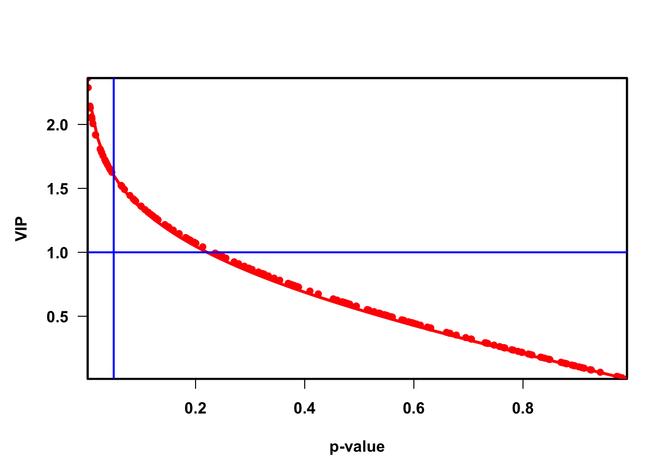

ttest_res <- t_fun(
  x = se_norm,
  group = "group",
  group_names = c("Mild", "Severe"))

m_results <- mergedResults(
  fc_result = fc_res,
  vip_result = vip_res$vip,
  test_result = ttest_res,
  group_names = c("Mild", "Severe"),
  group_labels = c("Mild", "Severe"))

head(m_results)

##   FeatureID         Block2                  Block FoldChange Log2FoldChange      VIP   CorPvalue Statistic      Pvalue AdjustedPvalue
## 1   M_42449 Mild vs Severe 14_Mild vs 19_Moderate  0.6571801     -0.6056393 2.362694 0.002247897 -3.498896 0.001881585      0.2132448
## 2   M_52446 Mild vs Severe 14_Mild vs 19_Moderate  0.7040861     -0.5061763 2.059461 0.009476225 -2.892892 0.008125613      0.2132448
## 3    M_1566 Mild vs Severe 14_Mild vs 19_Moderate  0.7161609     -0.4816443 2.143655 0.006556886 -3.077688 0.005431005      0.2132448
## 4   M_19263 Mild vs Severe 14_Mild vs 19_Moderate  0.7165011     -0.4809592 2.128317 0.007023483 -3.073546 0.005774977      0.2132448
## 5   M_42448 Mild vs Severe 14_Mild vs 19_Moderate  0.7577644     -0.4001788 2.006246 0.011828403 -2.793941 0.010215320      0.2132448
## 6   M_43761 Mild vs Severe 14_Mild vs 19_Moderate  0.8685495     -0.2033201 2.043515 0.010136007 -2.822338 0.009428795      0.2132448

4.3.4 Metabolites ID for Merged Results

HMDBID
KEGG ID: cpd_ID

get_metaboID <- function(
  x = ExprSet,
  dat,
  group_names,
  index_names = c("FoldChange", "Log2FoldChange", "VIP", "CorPvalue", "Pvalue", "AdjustedPvalue"),
  index_cutoff = c(1, 1, 1, 0.05, 0.05, 0.2)) {
  
  # x = ExprSet
  # dat = m_results
  # group_names = "Mild vs Severe"
  # index_names = c("Log2FoldChange", "AdjustedPvalue")
  # index_cutoff = c(0, 1)
  
  feature <- Biobase::fData(x)
  colnames(feature)[which(colnames(feature) == "SampleID HMDBID")] <- "HMDB"
  colnames(feature)[which(colnames(feature) == "KEGG")] <- "cpd_ID"
  colnames(feature)[which(colnames(feature) == "BIOCHEMICAL")] <- "Compounds"
  feature$HMDB <- gsub(",\\S+", "", feature$HMDB)
  
  temp_dat <- dat %>%
    dplyr::filter(Block2 %in% group_names) %>%
    dplyr::inner_join(feature %>%
                        tibble::rownames_to_column("FeatureID"),
                      by = "FeatureID")
  
  colnames(temp_dat)[which(colnames(temp_dat) == index_names[1])] <- "DA_index1"
  colnames(temp_dat)[which(colnames(temp_dat) == index_names[2])] <- "DA_index2"
  
  temp_dat_diff <- temp_dat %>%
    dplyr::filter(abs(DA_index1) > index_cutoff[1]) %>%
    dplyr::filter(DA_index2 < index_cutoff[2]) 
  
  if (nrow(temp_dat_diff) == 0) {
    stop("Beyond these thresholds, no significant metabolites were selected")
  }
  
  colnames(temp_dat_diff)[which(colnames(temp_dat_diff) == "DA_index1")] <- index_names[1]
  colnames(temp_dat_diff)[which(colnames(temp_dat_diff) == "DA_index2")] <- index_names[2]
  
  res <- temp_dat_diff 

  return(res)
}

m_results_ID <- get_metaboID(
  x = ExprSet,
  dat = m_results,
  group_names = "Mild vs Severe",
  index_names = c("Log2FoldChange", "AdjustedPvalue"),
  index_cutoff = c(0, 1))
  
head(m_results_ID)

##   FeatureID         Block2                  Block FoldChange Log2FoldChange      VIP   CorPvalue Statistic      Pvalue AdjustedPvalue
## 1   M_42449 Mild vs Severe 14_Mild vs 19_Moderate  0.6571801     -0.6056393 2.362694 0.002247897 -3.498896 0.001881585      0.2132448
## 2   M_52446 Mild vs Severe 14_Mild vs 19_Moderate  0.7040861     -0.5061763 2.059461 0.009476225 -2.892892 0.008125613      0.2132448
## 3    M_1566 Mild vs Severe 14_Mild vs 19_Moderate  0.7161609     -0.4816443 2.143655 0.006556886 -3.077688 0.005431005      0.2132448
## 4   M_19263 Mild vs Severe 14_Mild vs 19_Moderate  0.7165011     -0.4809592 2.128317 0.007023483 -3.073546 0.005774977      0.2132448
## 5   M_42448 Mild vs Severe 14_Mild vs 19_Moderate  0.7577644     -0.4001788 2.006246 0.011828403 -2.793941 0.010215320      0.2132448
## 6   M_43761 Mild vs Severe 14_Mild vs 19_Moderate  0.8685495     -0.2033201 2.043515 0.010136007 -2.822338 0.009428795      0.2132448
##                                 Compounds SUPER PATHWAY                               SUB PATHWAY COMP ID        PLATFORM CHEMICAL ID   RI     MASS
## 1 1-palmitoyl-2-linoleoyl-GPE (16:0/18:2)         Lipid             Phosphatidylethanolamine (PE)   42449  LC/MS Pos Late   100001870 2350 716.5225
## 2 1-stearoyl-2-linoleoyl-GPE (18:0/18:2)*         Lipid             Phosphatidylethanolamine (PE)   52446  LC/MS Pos Late   100008976 2575 744.5538
## 3                      3-aminoisobutyrate    Nucleotide Pyrimidine Metabolism, Thymine containing    1566 LC/MS Pos Early        1114 2190 104.0706
## 4    1-palmitoyl-2-oleoyl-GPE (16:0/18:1)         Lipid             Phosphatidylethanolamine (PE)   19263  LC/MS Pos Late        1526 2600 718.5381
## 5     1-stearoyl-2-oleoyl-GPE (18:0/18:1)         Lipid             Phosphatidylethanolamine (PE)   42448  LC/MS Pos Late   100001856 2950 746.5694
## 6                       2-aminoheptanoate         Lipid                         Fatty Acid, Amino   43761 LC/MS Pos Early   100004542 3160 146.1176
##   PUBCHEM                    CAS cpd_ID        HMDB
## 1 9546747                   <NA>   <NA> HMDB0005322
## 2 9546749                   <NA>   <NA> HMDB0008994
## 3   64956 10569-72-9;214139-20-5 C05145 HMDB0002166
## 4 5283496             26662-94-2   <NA> HMDB0005320
## 5 9546742                   <NA>   <NA> HMDB0008993
## 6  227939              1115-90-8   <NA> HMDB0094649

4.3.5 KEGG PATHWAY COMPOUND

KEGG pathway ID：request_kegg_pathway_info
KEGG pathway compound: request_kegg_pathway
data.frame with all pathway contained compounds id: 1st->pathwayID & 2nd->compoundID

get_kegg_pathway_compound <- function(
    org_id = c("hsa", "mmu")) {

  pathway_names <- request_kegg_pathway_info(organism = org_id)

  res <- data.frame()
  for (i in 1:nrow(pathway_names)) {
    # i = 12
    temp_pathway <- request_kegg_pathway(pathway_id = pathway_names$KEGG.ID[i])
    temp_colnames <- names(temp_pathway)

    if (all(c("COMPOUND", "ENTRY", "NAME", "CLASS", "PATHWAY_MAP") %in% temp_colnames)) {
      print(i)
      temp_compound <- temp_pathway$COMPOUND
      temp_class <- unlist(strsplit(temp_pathway$CLASS, "; "))
      temp_df1 <- data.frame(Pathway = temp_pathway$ENTRY,
                             NAME = temp_pathway$NAME,
                             #DESCRIPTION = temp_pathway$DESCRIPTION,
                             CLASS1 = temp_class[1],
                             CLASS2 = temp_class[2],
                             PATHWAY_MAP = temp_pathway$PATHWAY_MAP)
      temp_df2 <- data.frame(Pathway = rep(temp_pathway$ENTRY, length(temp_compound)),
                             COMPOUND = names(temp_compound),
                             COMPOUND_DESCRIPTION = temp_compound)

      temp_df <- temp_df1 %>%
        dplyr::full_join(temp_df2, by = "Pathway")

      res <- rbind(res, temp_df)
    }
  }

  return(res)
}

if (!dir.exists("./dataset/KEGG_COMPOUND_PATHWAY/")) {
  dir.create("./dataset/KEGG_COMPOUND_PATHWAY/", recursive = TRUE)
}

if (file.exists("./dataset/KEGG_COMPOUND_PATHWAY/KEGG_COMPOUND_PATHWAY_mmu.csv")) {
  kegg_compound <- read.csv("./dataset/KEGG_COMPOUND_PATHWAY/KEGG_COMPOUND_PATHWAY_mmu.csv")
} else {
  kegg_compound <- get_kegg_pathway_compound(org_id = "mmu")
  write.csv(kegg_compound, "./dataset/KEGG_COMPOUND_PATHWAY/KEGG_COMPOUND_PATHWAY_mmu.csv", row.names = F)
}

4.3.6 Functions related to Analysis

significant metabolites
enrichment analysis
plotting results

get_significant <- function(
    dat,
    group_names,
    lg2fc_cutoff = 0.5,
    pval_cutoff = 0.05,
    qval_cutoff = 0.3) {

  dat_group <- dat %>%
    dplyr::filter(Block2 %in% paste(group_names, collapse = " vs ")) %>%
    dplyr::distinct()
  
  # remove cp_id eq "-"
  dat_fa <- dat_group %>% 
    dplyr::filter(cpd_ID != "-")
  
  colnames(dat_fa)[which(colnames(dat_fa) == "Log2FoldChange")] <- "lg2fc" # Log2FoldChange (Median)
  colnames(dat_fa)[which(colnames(dat_fa) == "Pvalue")] <- "pval"
  colnames(dat_fa)[which(colnames(dat_fa) == "AdjustedPvalue")] <- "qval"
  
  # convert NA into 1
  dat_fa$qval[is.na(dat_fa$qval)] <- 1
  
  # enrichment by beta and Pvalue AdjustedPvalue
  dat_fa[which(dat_fa$lg2fc > lg2fc_cutoff &
              dat_fa$pval < pval_cutoff &
              dat_fa$qval < qval_cutoff),
      "EnrichedDir"] <- group_names[1]
  dat_fa[which(dat_fa$lg2fc < -lg2fc_cutoff &
              dat_fa$pval < pval_cutoff &
              dat_fa$qval < qval_cutoff),
      "EnrichedDir"] <- group_names[2]
  dat_fa[which(abs(dat_fa$lg2fc) <= lg2fc_cutoff |
              dat_fa$pval >= pval_cutoff |
              dat_fa$qval >= qval_cutoff),
      "EnrichedDir"] <- "Nonsignif"

  # dat status
  dat_fa$EnrichedDir <- factor(dat_fa$EnrichedDir,
                            levels = c(group_names[1], "Nonsignif", group_names[2]))
  df_status <- table(dat_fa$EnrichedDir) %>% data.frame() %>%
    stats::setNames(c("Group", "Number"))
  grp1_number <- with(df_status, df_status[Group %in% group_names[1], "Number"])
  grp2_number <- with(df_status, df_status[Group %in% group_names[2], "Number"])
  nsf_number <- with(df_status, df_status[Group %in% "Nonsignif", "Number"])
  legend_label <- c(paste0(group_names[1], " (", grp1_number, ")"),
                    paste0("Nonsignif", " (", nsf_number, ")"),
                    paste0(group_names[2], " (", grp2_number, ")"))

  # significant features
  dat_signif <- dat_fa %>%
    dplyr::arrange(lg2fc, pval, qval) %>%
    dplyr::filter(pval < pval_cutoff) %>%
    dplyr::filter(qval < qval_cutoff) %>%
    dplyr::filter(abs(lg2fc) > lg2fc_cutoff) %>%
    dplyr::select(FeatureID, Block, EnrichedDir, lg2fc, pval, qval, cpd_ID, everything()) %>%
    dplyr::mutate(FeatureID = gsub("\\.", "-", FeatureID))
  
  # print(table(dat_signif$EnrichedDir))

  res_up <- dat_signif %>% # enriched in 1st group
    dplyr::filter(EnrichedDir == group_names[1]) %>%
    dplyr::mutate(Status = "UpRegulated")

  res_down <- dat_signif %>% # enriched in 2st group
    dplyr::filter(EnrichedDir == group_names[2]) %>%
    dplyr::mutate(Status = "DownRegulated")

  res <- list(none = dat_fa %>%
                dplyr::select(FeatureID, Block, EnrichedDir, lg2fc, pval, qval, cpd_ID, everything()),
              all = dat_signif,
              up = res_up,
              down = res_down)

  return(res)
}

get_enrichment <- function(
    dat,
    ref = kegg_compound,
    direction = c("All", "DownRegulated", "UpRegulated"), # DownRegulated->1st group; UpRegulated->2nd group
    group_names,
    enrich_type = c("ORA", "GSEA"),
    lg2fc_cutoff = 0.5,
    pval_cutoff = 0.05,
    qval_cutoff = 0.3) {

  # dat = m_results_ID
  # ref = kegg_compound
  # direction = "none"
  # group_names = c("Mild", "Severe")
  # enrich_type = "GSEA"
  # lg2fc_cutoff = 0
  # pval_cutoff = 1
  # qval_cutoff = 1  
  
  temp_input <- get_significant(
    dat = dat,
    group_names = group_names,
    lg2fc_cutoff = lg2fc_cutoff,
    pval_cutoff = pval_cutoff,
    qval_cutoff = qval_cutoff)
  
  if (direction == "All") {
    inputdata <- temp_input$all
  } else if (direction == "UpRegulated") {
    inputdata <- temp_input$up
  } else if (direction == "DownRegulated") {
    inputdata <- temp_input$down
  } else if (direction == "none") {
    inputdata <- temp_input$none
  } 

  if (nrow(inputdata) == 0) {
    stop("Beyond these thresholds, no significant metabolites were selected")
  }  
  
  inputdata$cpd_ID <- gsub("\\s+\\|\\s+\\w+\\d+", "", inputdata$cpd_ID)
  inputdata$cpd_ID <- gsub(",\\S+", "", inputdata$cpd_ID)
  
  ref_cln <- ref %>%
    dplyr::select(PATHWAY_MAP, COMPOUND) %>%
    dplyr::rename(Pathway = PATHWAY_MAP)

  if (enrich_type == "ORA") {
    fit <- clusterProfiler::enricher(
                gene = inputdata$cpd_ID,
                pvalueCutoff = 0.05,
                pAdjustMethod = "BH",
                minGSSize = 10,
                maxGSSize = 500,
                qvalueCutoff = 0.2,
                TERM2GENE = ref_cln)
  } else if (enrich_type == "GSEA") {
    dat_GSEA <- inputdata %>%
      dplyr::arrange(desc(lg2fc))
    cpd_lg2fc <- dat_GSEA$lg2fc
    names(cpd_lg2fc) <- dat_GSEA$cpd_ID
    fit <- clusterProfiler::GSEA(
                geneList = cpd_lg2fc,
                pvalueCutoff = 0.05,
                pAdjustMethod = "BH",
                minGSSize = 10,
                maxGSSize = 500,
                TERM2GENE = ref_cln)
  }

  if (nrow(fit@result) != 0) {
    if (enrich_type == "ORA") {
      EA_res <- fit@result %>%
        dplyr::filter(!is.na(Description)) %>%
        dplyr::rename(CompoundRatio = GeneRatio,
                      CompoundID = geneID,
                      NAME = Description) %>%
        dplyr::select(ID, NAME, everything())      
    } else if (enrich_type == "GSEA") {
      EA_res <- fit@result %>%
        dplyr::filter(!is.na(Description)) %>%
        dplyr::rename(NAME = Description) %>%
        dplyr::select(ID, NAME, everything())       
    }
  } else {
    EA_res <- NULL
  }

  res <- list(data = inputdata,
              enrich = EA_res)

  return(res)
}

plot_enrichment <- function(
    inputdata,
    qval_cutoff = 0.05,
    topN = 10,
    plot_type = c("bubble", "bar"),
    enrich_type = c("ORA", "GSEA")) {


  if (nrow(inputdata) == 0) {
    stop("No pathway please check your input")
  }

  if (enrich_type == "ORA") {

    if (any(is.na(inputdata$qvalue))) {
      inputdata$qvalue <- inputdata$p.adjust
    }

    plotdata_temp <- inputdata %>%
      dplyr::select(ID, NAME, CompoundRatio, qvalue, Count) %>%
      dplyr::filter(qvalue < qval_cutoff)

    if (nrow(plotdata_temp) == 0) {
      stop("No pathway met the threshold of qvalue")
    }

    plotdata <- plotdata_temp %>%
      dplyr::slice(1:topN) %>%
      dplyr::mutate(qvalue = as.numeric(qvalue),
                    Count = as.numeric(Count)) %>%
      dplyr::group_by(ID) %>%
      dplyr::mutate(CompoundRatio1 = unlist(strsplit(CompoundRatio, "/"))[1],
                    CompoundRatio2 = unlist(strsplit(CompoundRatio, "/"))[2],
                    CompoundRatio = as.numeric(CompoundRatio1) / as.numeric(CompoundRatio2)) %>%
      dplyr::select(-all_of(c("CompoundRatio1", "CompoundRatio2"))) %>%
      dplyr::mutate(NAME = gsub(" - Mus musculus \\(house mouse\\)", "", NAME)) %>%
      dplyr::arrange(CompoundRatio)  %>%
      dplyr::rename(Yvalue = CompoundRatio)
    y_lab <- "CompoundRatio"
  } else if (enrich_type == "GSEA") {
    if (any(is.na(inputdata$qvalue))) {
      inputdata$qvalues <- inputdata$p.adjust
    }
    plotdata_temp <- inputdata %>%
      dplyr::select(ID, NAME, enrichmentScore, qvalues, setSize) %>% 
      dplyr::filter(qvalues < qval_cutoff)

    if (nrow(plotdata_temp) == 0) {
      stop("No pathway met the threshold of qvalue")
    }

    plotdata <- plotdata_temp %>%
      dplyr::slice(1:topN) %>%
      dplyr::rename(qvalue = qvalues,
                    Count = setSize) %>%
      dplyr::mutate(qvalue = as.numeric(qvalue),
                    Count = as.numeric(Count),
                    enrichmentScore = as.numeric(enrichmentScore)) %>%
      dplyr::mutate(NAME = gsub(" - Mus musculus \\(house mouse\\)", "", NAME)) %>%
      dplyr::arrange(enrichmentScore) %>%
      dplyr::rename(Yvalue = enrichmentScore)
    y_lab <- "enrichmentScore"
  }

  plotdata$NAME <- factor(plotdata$NAME, levels = as.character(plotdata$NAME))

  final_topN <- nrow(plotdata)

  if (plot_type == "bubble") {
    pl <- ggplot(plotdata, aes(x = NAME, y = Yvalue)) +
      geom_point(aes(size = Count, color = qvalue)) +
      coord_flip() +
      labs(x = "", y = y_lab, title = paste("Top", final_topN, "of Enrichment")) +
      theme_bw() +
      guides(size = guide_legend(order = 1),
             color = guide_legend(order = 2))+
      scale_color_gradientn(name = "q value",
                            colours = rainbow(5)) +
      theme(plot.title = element_text(face = 'bold', size = 12, hjust = .5),
            axis.title = element_text(face = 'bold', size = 11),
            axis.text.y = element_text(face = 'bold', size = 10),
            legend.position = "right")
  } else if (plot_type == "bar") {
    pl <- ggplot(plotdata, aes(x = NAME, y = Yvalue, fill = -log(qvalue))) +
      geom_bar(stat = "identity", position = position_dodge()) +
      coord_flip() +
      labs(x = "", y = y_lab, title = paste("Top", final_topN, "of Enrichment")) +
      theme_bw() +
      guides(fill = guide_legend(order = 1))+
      scale_color_gradientn(name = "-log10(q value)",
                            colours = rainbow(5)) +
      theme(plot.title = element_text(face = 'bold', size = 12, hjust = .5),
            axis.title = element_text(face = 'bold', size = 11),
            axis.text.y = element_text(face = 'bold', size = 10),
            legend.position = "right")
  }

  return(pl)
}

4.3.6.1 ORA

ORA: Enriched KEGG pathway for Down-Regulated Metabolites

Mild_Severe_ORA_Down <- get_enrichment(
  dat = m_results_ID,
  direction = "DownRegulated",
  group_names = c("Mild", "Severe"),
  enrich_type = "ORA", 
  lg2fc_cutoff = 0,
  pval_cutoff = 0.5,
  qval_cutoff = 1)

plot_enrichment(
  inputdata = Mild_Severe_ORA_Down$enrich,
  qval_cutoff = 0.5,
  topN = 10,
  plot_type = "bubble",
  enrich_type = "ORA")

head(Mild_Severe_ORA_Down$enrich)

##                                                                              ID                                    NAME CompoundRatio BgRatio
## Retrograde endocannabinoid signaling       Retrograde endocannabinoid signaling    Retrograde endocannabinoid signaling           1/5 19/3516
## Thermogenesis                                                     Thermogenesis                           Thermogenesis           1/5 23/3516
## Pentose phosphate pathway                             Pentose phosphate pathway               Pentose phosphate pathway           1/5 36/3516
## Histidine metabolism                                       Histidine metabolism                    Histidine metabolism           1/5 47/3516
## Phenylalanine metabolism                               Phenylalanine metabolism                Phenylalanine metabolism           1/5 49/3516
## Neuroactive ligand-receptor interaction Neuroactive ligand-receptor interaction Neuroactive ligand-receptor interaction           1/5 53/3516
##                                             pvalue   p.adjust     qvalue CompoundID Count
## Retrograde endocannabinoid signaling    0.02674395 0.08982828 0.07354362     C13856     1
## Thermogenesis                           0.03230064 0.08982828 0.07354362     C13856     1
## Pentose phosphate pathway               0.05018484 0.08982828 0.07354362     C00204     1
## Histidine metabolism                    0.06511021 0.08982828 0.07354362     C01152     1
## Phenylalanine metabolism                0.06780364 0.08982828 0.07354362     C05852     1
## Neuroactive ligand-receptor interaction 0.07317187 0.08982828 0.07354362     C13856     1

4.3.6.2 GSEA

GSEA: Enriched KEGG pathway for all Metabolites whose rank by log2foldchange

Mild_Severe_GSEA <- get_enrichment(
  dat = m_results_ID,
  direction = "none",
  group_names = c("Mild", "Severe"),
  enrich_type = "GSEA", 
  lg2fc_cutoff = 0,
  pval_cutoff = 0.5,
  qval_cutoff = 1)

# plot_enrichment(
#   inputdata = Mild_Severe_GSEA$enrich,
#   qval_cutoff = 0.5,
#   topN = 10,
#   plot_type = "bubble",
#   enrich_type = "GSEA")
# 
# head(Mild_Severe_GSEA$enrich)

4.4 Session info

devtools::session_info()

## ─ Session info ─────────────────────────────────────────────────────────────────────────────────────────────────────────────────────────────────────
##  setting  value
##  version  R version 4.1.3 (2022-03-10)
##  os       macOS Monterey 12.2.1
##  system   x86_64, darwin17.0
##  ui       RStudio
##  language (EN)
##  collate  en_US.UTF-8
##  ctype    en_US.UTF-8
##  tz       Asia/Shanghai
##  date     2023-12-07
##  rstudio  2023.09.0+463 Desert Sunflower (desktop)
##  pandoc   3.1.1 @ /Applications/RStudio.app/Contents/Resources/app/quarto/bin/tools/ (via rmarkdown)
## 
## ─ Packages ─────────────────────────────────────────────────────────────────────────────────────────────────────────────────────────────────────────
##  package              * version    date (UTC) lib source
##  abind                  1.4-5      2016-07-21 [2] CRAN (R 4.1.0)
##  ade4                   1.7-22     2023-02-06 [2] CRAN (R 4.1.2)
##  affy                   1.72.0     2021-10-26 [2] Bioconductor
##  affyio                 1.64.0     2021-10-26 [2] Bioconductor
##  annotate               1.72.0     2021-10-26 [2] Bioconductor
##  AnnotationDbi        * 1.60.2     2023-03-10 [2] Bioconductor
##  ape                    5.7-1      2023-03-13 [2] CRAN (R 4.1.2)
##  aplot                  0.1.10     2023-03-08 [2] CRAN (R 4.1.2)
##  attempt                0.3.1      2020-05-03 [2] CRAN (R 4.1.0)
##  backports              1.4.1      2021-12-13 [2] CRAN (R 4.1.0)
##  base64enc              0.1-3      2015-07-28 [2] CRAN (R 4.1.0)
##  Biobase              * 2.54.0     2021-10-26 [2] Bioconductor
##  BiocGenerics         * 0.40.0     2021-10-26 [2] Bioconductor
##  BiocManager            1.30.21    2023-06-10 [2] CRAN (R 4.1.3)
##  BiocParallel           1.28.3     2021-12-09 [2] Bioconductor
##  biomformat             1.22.0     2021-10-26 [2] Bioconductor
##  Biostrings             2.62.0     2021-10-26 [2] Bioconductor
##  bit                    4.0.5      2022-11-15 [2] CRAN (R 4.1.2)
##  bit64                  4.0.5      2020-08-30 [2] CRAN (R 4.1.0)
##  bitops                 1.0-7      2021-04-24 [2] CRAN (R 4.1.0)
##  blob                   1.2.4      2023-03-17 [2] CRAN (R 4.1.2)
##  bookdown               0.34       2023-05-09 [2] CRAN (R 4.1.2)
##  broom                  1.0.5      2023-06-09 [2] CRAN (R 4.1.3)
##  bslib                  0.6.0      2023-11-21 [1] CRAN (R 4.1.3)
##  cachem                 1.0.8      2023-05-01 [2] CRAN (R 4.1.2)
##  Cairo                  1.6-0      2022-07-05 [2] CRAN (R 4.1.2)
##  callr                  3.7.3      2022-11-02 [2] CRAN (R 4.1.2)
##  car                    3.1-2      2023-03-30 [2] CRAN (R 4.1.2)
##  carData                3.0-5      2022-01-06 [2] CRAN (R 4.1.2)
##  caret                  6.0-94     2023-03-21 [2] CRAN (R 4.1.2)
##  caTools                1.18.2     2021-03-28 [2] CRAN (R 4.1.0)
##  cellranger             1.1.0      2016-07-27 [2] CRAN (R 4.1.0)
##  checkmate              2.2.0      2023-04-27 [2] CRAN (R 4.1.2)
##  circlize               0.4.15     2022-05-10 [2] CRAN (R 4.1.2)
##  class                  7.3-22     2023-05-03 [2] CRAN (R 4.1.2)
##  cli                    3.6.1      2023-03-23 [2] CRAN (R 4.1.2)
##  clue                   0.3-64     2023-01-31 [2] CRAN (R 4.1.2)
##  cluster              * 2.1.4      2022-08-22 [2] CRAN (R 4.1.2)
##  clusterProfiler      * 4.2.2      2022-01-13 [2] Bioconductor
##  codetools              0.2-19     2023-02-01 [2] CRAN (R 4.1.2)
##  coin                   1.4-2      2021-10-08 [2] CRAN (R 4.1.0)
##  colorspace             2.1-0      2023-01-23 [2] CRAN (R 4.1.2)
##  ComplexHeatmap         2.10.0     2021-10-26 [2] Bioconductor
##  config                 0.3.1      2020-12-17 [2] CRAN (R 4.1.0)
##  corpcor                1.6.10     2021-09-16 [2] CRAN (R 4.1.0)
##  cowplot                1.1.1      2020-12-30 [2] CRAN (R 4.1.0)
##  crayon                 1.5.2      2022-09-29 [2] CRAN (R 4.1.2)
##  crmn                   0.0.21     2020-02-10 [2] CRAN (R 4.1.0)
##  curl                   5.0.1      2023-06-07 [2] CRAN (R 4.1.3)
##  data.table             1.14.8     2023-02-17 [2] CRAN (R 4.1.2)
##  DBI                    1.1.3      2022-06-18 [2] CRAN (R 4.1.2)
##  DelayedArray           0.20.0     2021-10-26 [2] Bioconductor
##  dendextend           * 1.17.1     2023-03-25 [2] CRAN (R 4.1.2)
##  DESeq2                 1.34.0     2021-10-26 [2] Bioconductor
##  devtools               2.4.5      2022-10-11 [2] CRAN (R 4.1.2)
##  digest                 0.6.33     2023-07-07 [1] CRAN (R 4.1.3)
##  DO.db                  2.9        2022-04-11 [2] Bioconductor
##  doParallel             1.0.17     2022-02-07 [2] CRAN (R 4.1.2)
##  doRNG                  1.8.6      2023-01-16 [2] CRAN (R 4.1.2)
##  DOSE                   3.20.1     2021-11-18 [2] Bioconductor
##  doSNOW                 1.0.20     2022-02-04 [2] CRAN (R 4.1.2)
##  downloader             0.4        2015-07-09 [2] CRAN (R 4.1.0)
##  dplyr                * 1.1.2      2023-04-20 [2] CRAN (R 4.1.2)
##  DT                     0.28       2023-05-18 [2] CRAN (R 4.1.3)
##  dynamicTreeCut         1.63-1     2016-03-11 [2] CRAN (R 4.1.0)
##  e1071                  1.7-13     2023-02-01 [2] CRAN (R 4.1.2)
##  edgeR                  3.36.0     2021-10-26 [2] Bioconductor
##  ellipse                0.4.5      2023-04-05 [2] CRAN (R 4.1.2)
##  ellipsis               0.3.2      2021-04-29 [2] CRAN (R 4.1.0)
##  enrichplot             1.14.2     2022-02-24 [2] Bioconductor
##  evaluate               0.21       2023-05-05 [2] CRAN (R 4.1.2)
##  factoextra           * 1.0.7      2020-04-01 [2] CRAN (R 4.1.0)
##  fansi                  1.0.4      2023-01-22 [2] CRAN (R 4.1.2)
##  farver                 2.1.1      2022-07-06 [2] CRAN (R 4.1.2)
##  fastcluster            1.2.3      2021-05-24 [2] CRAN (R 4.1.0)
##  fastmap                1.1.1      2023-02-24 [2] CRAN (R 4.1.2)
##  fastmatch              1.1-3      2021-07-23 [2] CRAN (R 4.1.0)
##  fdrtool                1.2.17     2021-11-13 [2] CRAN (R 4.1.0)
##  fgsea                  1.20.0     2021-10-26 [2] Bioconductor
##  filematrix             1.3        2018-02-27 [2] CRAN (R 4.1.0)
##  foreach                1.5.2      2022-02-02 [2] CRAN (R 4.1.2)
##  foreign                0.8-84     2022-12-06 [2] CRAN (R 4.1.2)
##  forestplot             3.1.1      2022-12-06 [2] CRAN (R 4.1.2)
##  Formula                1.2-5      2023-02-24 [2] CRAN (R 4.1.2)
##  fs                     1.6.2      2023-04-25 [2] CRAN (R 4.1.2)
##  furrr                  0.3.1      2022-08-15 [2] CRAN (R 4.1.2)
##  future                 1.33.0     2023-07-01 [2] CRAN (R 4.1.3)
##  future.apply           1.11.0     2023-05-21 [2] CRAN (R 4.1.3)
##  genefilter             1.76.0     2021-10-26 [2] Bioconductor
##  geneplotter            1.72.0     2021-10-26 [2] Bioconductor
##  generics               0.1.3      2022-07-05 [2] CRAN (R 4.1.2)
##  GenomeInfoDb         * 1.30.1     2022-01-30 [2] Bioconductor
##  GenomeInfoDbData       1.2.7      2022-03-09 [2] Bioconductor
##  GenomicRanges        * 1.46.1     2021-11-18 [2] Bioconductor
##  GetoptLong             1.0.5      2020-12-15 [2] CRAN (R 4.1.0)
##  ggforce                0.4.1      2022-10-04 [2] CRAN (R 4.1.2)
##  ggfun                  0.1.1      2023-06-24 [2] CRAN (R 4.1.3)
##  ggplot2              * 3.4.2      2023-04-03 [2] CRAN (R 4.1.2)
##  ggplotify              0.1.1      2023-06-27 [2] CRAN (R 4.1.3)
##  ggpubr                 0.6.0      2023-02-10 [2] CRAN (R 4.1.2)
##  ggraph               * 2.1.0.9000 2023-07-11 [1] Github (thomasp85/ggraph@febab71)
##  ggrepel                0.9.3      2023-02-03 [2] CRAN (R 4.1.2)
##  ggsignif               0.6.4      2022-10-13 [2] CRAN (R 4.1.2)
##  ggtree                 3.2.1      2021-11-16 [2] Bioconductor
##  glasso                 1.11       2019-10-01 [2] CRAN (R 4.1.0)
##  glmnet               * 4.1-7      2023-03-23 [2] CRAN (R 4.1.2)
##  GlobalOptions          0.1.2      2020-06-10 [2] CRAN (R 4.1.0)
##  globals                0.16.2     2022-11-21 [2] CRAN (R 4.1.2)
##  globaltest             5.48.0     2021-10-26 [2] Bioconductor
##  glue                 * 1.6.2      2022-02-24 [2] CRAN (R 4.1.2)
##  Gmisc                * 3.0.2      2023-03-13 [2] CRAN (R 4.1.2)
##  gmm                    1.8        2023-06-06 [2] CRAN (R 4.1.3)
##  gmp                    0.7-1      2023-02-07 [2] CRAN (R 4.1.2)
##  GO.db                  3.14.0     2022-04-11 [2] Bioconductor
##  golem                  0.4.1      2023-06-05 [2] CRAN (R 4.1.3)
##  GOSemSim               2.20.0     2021-10-26 [2] Bioconductor
##  gower                  1.0.1      2022-12-22 [2] CRAN (R 4.1.2)
##  gplots                 3.1.3      2022-04-25 [2] CRAN (R 4.1.2)
##  graphlayouts           1.0.0      2023-05-01 [2] CRAN (R 4.1.2)
##  gridExtra              2.3        2017-09-09 [2] CRAN (R 4.1.0)
##  gridGraphics           0.5-1      2020-12-13 [2] CRAN (R 4.1.0)
##  gtable                 0.3.3      2023-03-21 [2] CRAN (R 4.1.2)
##  gtools                 3.9.4      2022-11-27 [2] CRAN (R 4.1.2)
##  hardhat                1.3.0      2023-03-30 [2] CRAN (R 4.1.2)
##  highr                  0.10       2022-12-22 [2] CRAN (R 4.1.2)
##  Hmisc                  5.1-0      2023-05-08 [2] CRAN (R 4.1.2)
##  hms                    1.1.3      2023-03-21 [2] CRAN (R 4.1.2)
##  htmlTable            * 2.4.1      2022-07-07 [2] CRAN (R 4.1.2)
##  htmltools              0.5.7      2023-11-03 [1] CRAN (R 4.1.3)
##  htmlwidgets            1.6.2      2023-03-17 [2] CRAN (R 4.1.2)
##  httpuv                 1.6.11     2023-05-11 [2] CRAN (R 4.1.3)
##  httr                 * 1.4.6      2023-05-08 [2] CRAN (R 4.1.2)
##  huge                   1.3.5      2021-06-30 [2] CRAN (R 4.1.0)
##  igraph                 1.5.0      2023-06-16 [1] CRAN (R 4.1.3)
##  impute                 1.68.0     2021-10-26 [2] Bioconductor
##  imputeLCMD             2.1        2022-06-10 [2] CRAN (R 4.1.2)
##  ipred                  0.9-14     2023-03-09 [2] CRAN (R 4.1.2)
##  IRanges              * 2.28.0     2021-10-26 [2] Bioconductor
##  irlba                  2.3.5.1    2022-10-03 [2] CRAN (R 4.1.2)
##  iterators              1.0.14     2022-02-05 [2] CRAN (R 4.1.2)
##  itertools              0.1-3      2014-03-12 [2] CRAN (R 4.1.0)
##  jpeg                   0.1-10     2022-11-29 [2] CRAN (R 4.1.2)
##  jquerylib              0.1.4      2021-04-26 [2] CRAN (R 4.1.0)
##  jsonlite               1.8.7      2023-06-29 [2] CRAN (R 4.1.3)
##  KEGGREST               1.34.0     2021-10-26 [2] Bioconductor
##  KernSmooth             2.23-22    2023-07-10 [2] CRAN (R 4.1.3)
##  knitr                  1.43       2023-05-25 [2] CRAN (R 4.1.3)
##  labeling               0.4.2      2020-10-20 [2] CRAN (R 4.1.0)
##  later                  1.3.1      2023-05-02 [2] CRAN (R 4.1.2)
##  lattice                0.21-8     2023-04-05 [2] CRAN (R 4.1.2)
##  lava                   1.7.2.1    2023-02-27 [2] CRAN (R 4.1.2)
##  lavaan                 0.6-15     2023-03-14 [2] CRAN (R 4.1.2)
##  lazyeval               0.2.2      2019-03-15 [2] CRAN (R 4.1.0)
##  libcoin                1.0-9      2021-09-27 [2] CRAN (R 4.1.0)
##  lifecycle              1.0.3      2022-10-07 [2] CRAN (R 4.1.2)
##  limma                  3.50.3     2022-04-07 [2] Bioconductor
##  listenv                0.9.0      2022-12-16 [2] CRAN (R 4.1.2)
##  locfit                 1.5-9.8    2023-06-11 [2] CRAN (R 4.1.3)
##  lubridate              1.9.2      2023-02-10 [2] CRAN (R 4.1.2)
##  magrittr             * 2.0.3      2022-03-30 [2] CRAN (R 4.1.2)
##  MALDIquant             1.22.1     2023-03-20 [2] CRAN (R 4.1.2)
##  MASS                   7.3-60     2023-05-04 [2] CRAN (R 4.1.2)
##  massdatabase         * 1.0.7      2023-05-30 [2] gitlab (jaspershen/massdatabase@df83e93)
##  massdataset          * 1.0.24     2023-05-30 [2] gitlab (jaspershen/massdataset@b397116)
##  masstools            * 1.0.10     2023-05-30 [2] gitlab (jaspershen/masstools@b3c73bc)
##  Matrix               * 1.6-0      2023-07-08 [2] CRAN (R 4.1.3)
##  MatrixGenerics       * 1.6.0      2021-10-26 [2] Bioconductor
##  matrixStats          * 1.0.0      2023-06-02 [2] CRAN (R 4.1.3)
##  memoise                2.0.1      2021-11-26 [2] CRAN (R 4.1.0)
##  MetaboAnalystR       * 3.2.0      2022-06-28 [2] Github (xia-lab/MetaboAnalystR@892a31b)
##  metagenomeSeq          1.36.0     2021-10-26 [2] Bioconductor
##  metid                * 1.2.26     2023-05-30 [2] gitlab (jaspershen/metid@6bde121)
##  metpath              * 1.0.5      2023-05-30 [2] gitlab (jaspershen/metpath@adcad4f)
##  mgcv                   1.8-42     2023-03-02 [2] CRAN (R 4.1.2)
##  MicrobiomeProfiler   * 1.0.0      2021-10-26 [2] Bioconductor
##  mime                   0.12       2021-09-28 [2] CRAN (R 4.1.0)
##  miniUI                 0.1.1.1    2018-05-18 [2] CRAN (R 4.1.0)
##  missForest             1.5        2022-04-14 [2] CRAN (R 4.1.2)
##  mixedCCA               1.6.2      2022-09-09 [2] CRAN (R 4.1.2)
##  mixOmics               6.18.1     2021-11-18 [2] Bioconductor (R 4.1.2)
##  mnormt                 2.1.1      2022-09-26 [2] CRAN (R 4.1.2)
##  ModelMetrics           1.2.2.2    2020-03-17 [2] CRAN (R 4.1.0)
##  modeltools             0.2-23     2020-03-05 [2] CRAN (R 4.1.0)
##  MsCoreUtils            1.6.2      2022-02-24 [2] Bioconductor
##  MSnbase              * 2.20.4     2022-01-16 [2] Bioconductor
##  multcomp               1.4-25     2023-06-20 [2] CRAN (R 4.1.3)
##  multtest               2.50.0     2021-10-26 [2] Bioconductor
##  munsell                0.5.0      2018-06-12 [2] CRAN (R 4.1.0)
##  mvtnorm                1.2-2      2023-06-08 [2] CRAN (R 4.1.3)
##  mzID                   1.32.0     2021-10-26 [2] Bioconductor
##  mzR                  * 2.28.0     2021-10-27 [2] Bioconductor
##  ncdf4                  1.21       2023-01-07 [2] CRAN (R 4.1.2)
##  NetCoMi              * 1.0.3      2022-07-14 [2] Github (stefpeschel/NetCoMi@d4d80d3)
##  nlme                   3.1-162    2023-01-31 [2] CRAN (R 4.1.2)
##  nnet                   7.3-19     2023-05-03 [2] CRAN (R 4.1.2)
##  norm                   1.0-11.1   2023-06-18 [2] CRAN (R 4.1.3)
##  openxlsx               4.2.5.2    2023-02-06 [2] CRAN (R 4.1.2)
##  org.Mm.eg.db         * 3.14.0     2022-11-23 [2] Bioconductor
##  parallelly             1.36.0     2023-05-26 [2] CRAN (R 4.1.3)
##  patchwork              1.1.2      2022-08-19 [2] CRAN (R 4.1.2)
##  pbapply                1.7-2      2023-06-27 [2] CRAN (R 4.1.3)
##  pbivnorm               0.6.0      2015-01-23 [2] CRAN (R 4.1.0)
##  pcaMethods             1.86.0     2021-10-26 [2] Bioconductor
##  pcaPP                  2.0-3      2022-10-24 [2] CRAN (R 4.1.2)
##  permute                0.9-7      2022-01-27 [2] CRAN (R 4.1.2)
##  phyloseq               1.38.0     2021-10-26 [2] Bioconductor
##  pillar                 1.9.0      2023-03-22 [2] CRAN (R 4.1.2)
##  pkgbuild               1.4.2      2023-06-26 [2] CRAN (R 4.1.3)
##  pkgconfig              2.0.3      2019-09-22 [2] CRAN (R 4.1.0)
##  pkgload                1.3.2.1    2023-07-08 [2] CRAN (R 4.1.3)
##  plotly               * 4.10.2     2023-06-03 [2] CRAN (R 4.1.3)
##  plyr                   1.8.8      2022-11-11 [2] CRAN (R 4.1.2)
##  png                    0.1-8      2022-11-29 [2] CRAN (R 4.1.2)
##  polyclip               1.10-4     2022-10-20 [2] CRAN (R 4.1.2)
##  POMA                 * 1.7.2      2022-07-26 [2] Github (pcastellanoescuder/POMA@bc8a972)
##  preprocessCore         1.56.0     2021-10-26 [2] Bioconductor
##  prettyunits            1.1.1      2020-01-24 [2] CRAN (R 4.1.0)
##  pROC                   1.18.4     2023-07-06 [2] CRAN (R 4.1.3)
##  processx               3.8.2      2023-06-30 [2] CRAN (R 4.1.3)
##  prodlim                2023.03.31 2023-04-02 [2] CRAN (R 4.1.2)
##  profvis                0.3.8      2023-05-02 [2] CRAN (R 4.1.2)
##  progress               1.2.2      2019-05-16 [2] CRAN (R 4.1.0)
##  promises               1.2.0.1    2021-02-11 [2] CRAN (R 4.1.0)
##  ProtGenerics         * 1.26.0     2021-10-26 [2] Bioconductor
##  proxy                  0.4-27     2022-06-09 [2] CRAN (R 4.1.2)
##  ps                     1.7.5      2023-04-18 [2] CRAN (R 4.1.2)
##  psych                  2.3.6      2023-06-21 [2] CRAN (R 4.1.3)
##  pulsar                 0.3.10     2023-01-26 [2] CRAN (R 4.1.2)
##  purrr                  1.0.1      2023-01-10 [2] CRAN (R 4.1.2)
##  qgraph                 1.9.5      2023-05-16 [2] CRAN (R 4.1.3)
##  qs                     0.25.5     2023-02-22 [2] CRAN (R 4.1.2)
##  quadprog               1.5-8      2019-11-20 [2] CRAN (R 4.1.0)
##  qvalue                 2.26.0     2021-10-26 [2] Bioconductor
##  R6                     2.5.1      2021-08-19 [2] CRAN (R 4.1.0)
##  ragg                   1.2.5      2023-01-12 [2] CRAN (R 4.1.2)
##  randomForest           4.7-1.1    2022-05-23 [2] CRAN (R 4.1.2)
##  RankProd               3.20.0     2021-10-26 [2] Bioconductor
##  RApiSerialize          0.1.2      2022-08-25 [2] CRAN (R 4.1.2)
##  rARPACK                0.11-0     2016-03-10 [2] CRAN (R 4.1.0)
##  rbibutils              2.2.13     2023-01-13 [2] CRAN (R 4.1.2)
##  RColorBrewer           1.1-3      2022-04-03 [2] CRAN (R 4.1.2)
##  Rcpp                 * 1.0.11     2023-07-06 [1] CRAN (R 4.1.3)
##  RcppParallel           5.1.7      2023-02-27 [2] CRAN (R 4.1.2)
##  RCurl                  1.98-1.12  2023-03-27 [2] CRAN (R 4.1.2)
##  Rdisop                 1.54.0     2021-10-26 [2] Bioconductor
##  Rdpack                 2.4        2022-07-20 [2] CRAN (R 4.1.2)
##  readr                  2.1.4      2023-02-10 [2] CRAN (R 4.1.2)
##  readxl               * 1.4.3      2023-07-06 [2] CRAN (R 4.1.3)
##  recipes                1.0.6      2023-04-25 [2] CRAN (R 4.1.2)
##  remotes                2.4.2      2021-11-30 [2] CRAN (R 4.1.0)
##  reshape2               1.4.4      2020-04-09 [2] CRAN (R 4.1.0)
##  rhdf5                  2.38.1     2022-03-10 [2] Bioconductor
##  rhdf5filters           1.6.0      2021-10-26 [2] Bioconductor
##  Rhdf5lib               1.16.0     2021-10-26 [2] Bioconductor
##  rjson                  0.2.21     2022-01-09 [2] CRAN (R 4.1.2)
##  rlang                  1.1.1      2023-04-28 [1] CRAN (R 4.1.2)
##  rmarkdown              2.23       2023-07-01 [2] CRAN (R 4.1.3)
##  Rmpfr                  0.9-2      2023-04-22 [2] CRAN (R 4.1.2)
##  rngtools               1.5.2      2021-09-20 [2] CRAN (R 4.1.0)
##  rootSolve              1.8.2.3    2021-09-29 [2] CRAN (R 4.1.0)
##  ropls                * 1.26.4     2022-01-11 [2] Bioconductor
##  rpart                  4.1.19     2022-10-21 [2] CRAN (R 4.1.2)
##  Rserve               * 1.8-11     2022-11-28 [2] CRAN (R 4.1.2)
##  RSpectra               0.16-1     2022-04-24 [2] CRAN (R 4.1.2)
##  RSQLite                2.3.1      2023-04-03 [2] CRAN (R 4.1.2)
##  rstatix                0.7.2      2023-02-01 [2] CRAN (R 4.1.2)
##  rstudioapi             0.15.0     2023-07-07 [2] CRAN (R 4.1.3)
##  rvest                  1.0.3      2022-08-19 [2] CRAN (R 4.1.2)
##  S4Vectors            * 0.32.4     2022-03-29 [2] Bioconductor
##  sandwich               3.0-2      2022-06-15 [2] CRAN (R 4.1.2)
##  sass                   0.4.6      2023-05-03 [2] CRAN (R 4.1.2)
##  scales                 1.2.1      2022-08-20 [2] CRAN (R 4.1.2)
##  scatterpie             0.2.1      2023-06-07 [2] CRAN (R 4.1.3)
##  scrime                 1.3.5      2018-12-01 [2] CRAN (R 4.1.0)
##  sessioninfo            1.2.2      2021-12-06 [2] CRAN (R 4.1.0)
##  shadowtext             0.1.2      2022-04-22 [2] CRAN (R 4.1.2)
##  shape                  1.4.6      2021-05-19 [2] CRAN (R 4.1.0)
##  shiny                  1.7.4.1    2023-07-06 [2] CRAN (R 4.1.3)
##  shinycustomloader      0.9.0      2018-03-27 [2] CRAN (R 4.1.0)
##  shinyWidgets           0.7.6      2023-01-08 [2] CRAN (R 4.1.2)
##  siggenes               1.68.0     2021-10-26 [2] Bioconductor
##  snow                   0.4-4      2021-10-27 [2] CRAN (R 4.1.0)
##  SpiecEasi            * 1.1.2      2022-07-14 [2] Github (zdk123/SpiecEasi@c463727)
##  SPRING               * 1.0.4      2022-08-03 [2] Github (GraceYoon/SPRING@3d641a4)
##  stringdist             0.9.10     2022-11-07 [2] CRAN (R 4.1.2)
##  stringfish             0.15.8     2023-05-30 [2] CRAN (R 4.1.3)
##  stringi                1.7.12     2023-01-11 [2] CRAN (R 4.1.2)
##  stringr                1.5.0      2022-12-02 [2] CRAN (R 4.1.2)
##  SummarizedExperiment * 1.24.0     2021-10-26 [2] Bioconductor
##  survival               3.5-5      2023-03-12 [2] CRAN (R 4.1.2)
##  systemfonts            1.0.4      2022-02-11 [2] CRAN (R 4.1.2)
##  textshaping            0.3.6      2021-10-13 [2] CRAN (R 4.1.0)
##  TH.data                1.1-2      2023-04-17 [2] CRAN (R 4.1.2)
##  tibble               * 3.2.1      2023-03-20 [2] CRAN (R 4.1.2)
##  tidygraph              1.2.3      2023-02-01 [2] CRAN (R 4.1.2)
##  tidyr                  1.3.0      2023-01-24 [2] CRAN (R 4.1.2)
##  tidyselect             1.2.0      2022-10-10 [2] CRAN (R 4.1.2)
##  tidytree               0.4.2      2022-12-18 [2] CRAN (R 4.1.2)
##  timechange             0.2.0      2023-01-11 [2] CRAN (R 4.1.2)
##  timeDate               4022.108   2023-01-07 [2] CRAN (R 4.1.2)
##  tmvtnorm               1.5        2022-03-22 [2] CRAN (R 4.1.2)
##  treeio                 1.18.1     2021-11-14 [2] Bioconductor
##  tweenr                 2.0.2      2022-09-06 [2] CRAN (R 4.1.2)
##  tzdb                   0.4.0      2023-05-12 [2] CRAN (R 4.1.3)
##  urlchecker             1.0.1      2021-11-30 [2] CRAN (R 4.1.0)
##  usethis                2.2.2      2023-07-06 [2] CRAN (R 4.1.3)
##  utf8                   1.2.3      2023-01-31 [2] CRAN (R 4.1.2)
##  vctrs                  0.6.3      2023-06-14 [1] CRAN (R 4.1.3)
##  vegan                  2.6-4      2022-10-11 [2] CRAN (R 4.1.2)
##  VGAM                   1.1-8      2023-03-09 [2] CRAN (R 4.1.2)
##  viridis                0.6.3      2023-05-03 [2] CRAN (R 4.1.2)
##  viridisLite            0.4.2      2023-05-02 [2] CRAN (R 4.1.2)
##  vsn                    3.62.0     2021-10-26 [2] Bioconductor
##  WGCNA                  1.72-1     2023-01-18 [2] CRAN (R 4.1.2)
##  withr                  2.5.0      2022-03-03 [2] CRAN (R 4.1.2)
##  Wrench                 1.12.0     2021-10-26 [2] Bioconductor
##  xfun                   0.40       2023-08-09 [1] CRAN (R 4.1.3)
##  XMAS2                * 2.2.0      2023-12-06 [1] local
##  XML                    3.99-0.14  2023-03-19 [2] CRAN (R 4.1.2)
##  xml2                   1.3.5      2023-07-06 [2] CRAN (R 4.1.3)
##  xtable                 1.8-4      2019-04-21 [2] CRAN (R 4.1.0)
##  XVector                0.34.0     2021-10-26 [2] Bioconductor
##  yaml                   2.3.7      2023-01-23 [2] CRAN (R 4.1.2)
##  yulab.utils            0.0.6      2022-12-20 [2] CRAN (R 4.1.2)
##  zip                    2.3.0      2023-04-17 [2] CRAN (R 4.1.2)
##  zlibbioc               1.40.0     2021-10-26 [2] Bioconductor
##  zoo                    1.8-12     2023-04-13 [2] CRAN (R 4.1.2)
## 
##  [1] /Users/zouhua/Library/R/x86_64/4.1/library
##  [2] /Library/Frameworks/R.framework/Versions/4.1/Resources/library
## 
## ────────────────────────────────────────────────────────────────────────────────────────────────────────────────────────────────────────────────────