Chapter 2 Data Processing
Although the horrible experience of data analysis by using MetaboAnalystR R package (Pang et al. 2020), its thought of data processing are very useful. Therefore, this template is based on the workflow from MetaboAnalystR.
We integrated R packages and our own scripts to build the data analysis template on metabolomic data. Particularly, we thanks very much for POMA R package (Castellano-Escuder et al. 2021). POMA is a flexible data cleaning and statistical analysis processes in one comprehensible and user-friendly R package.
2.2 Importing data
The dataset is from the Zeybel-2022 published paper (Zeybel et al. 2022).
- features table
## # A tibble: 6 × 67
##   BIOCHEMICAL `SUPER PATHWAY` `SUB PATHWAY` `COMP ID` PLATFORM `CHEMICAL ID`    RI  MASS PUBCHEM CAS   KEGG  `SampleID HMDBID` P101001 P101012 P101030
##   <chr>       <chr>           <chr>             <dbl> <chr>            <dbl> <dbl> <dbl> <chr>   <chr> <chr> <chr>               <dbl>   <dbl>   <dbl>
## 1 (14 or 15)… Lipid           Fatty Acid, …     38768 LC/MS N…     100002945  5695  269. 8181;1… <NA>  C169… HMDB0061859        5.11e7  5.12e7  3.84e7
## 2 (16 or 17)… Lipid           Fatty Acid, …     38296 LC/MS N…     100002356  5993  297. 3083779 2724… <NA>  HMDB0037397        5.11e6  6.00e6  2.86e6
## 3 (2 or 3)-d… Lipid           Medium Chain…     63436 LC/MS N…     100021502  4990  169. <NA>    <NA>  <NA>  <NA>               7.57e5  5.98e5  3.67e5
## 4 (2,4 or 2,… Xenobiotics     Food Compone…     62533 LC/MS N…     100020519  3474  201. <NA>    <NA>  <NA>  <NA>              NA      NA       5.64e5
## 5 (N(1) + N(… Amino Acid      Polyamine Me…     57814 LC/MS P…     100016038  3080  188. 123689… <NA>  C006… HMDB0001276,HMDB…  2.82e5  2.49e5  2.31e5
## 6 (R)-3-hydr… Lipid           Fatty Acid M…     43264 LC/MS P…     100003926  2400  248. 534816… <NA>  <NA>  HMDB0013127       NA      NA      NA
## # ℹ 52 more variables: P101031 <dbl>, P101050 <dbl>, P101059 <dbl>, P101071 <dbl>, P101072 <dbl>, P101084 <dbl>, P101003 <dbl>, P101004 <dbl>,
## #   P101013 <dbl>, P101016 <dbl>, P101017 <dbl>, P101038 <dbl>, P101051 <dbl>, P101061 <dbl>, P101062 <dbl>, P101074 <dbl>, P101075 <dbl>,
## #   P101076 <dbl>, P101085 <dbl>, P101088 <dbl>, P101007 <dbl>, P101018 <dbl>, P101019 <dbl>, P101041 <dbl>, P101052 <dbl>, P101064 <dbl>,
## #   P101065 <dbl>, P101077 <dbl>, P101090 <dbl>, P101094 <dbl>, P101009 <dbl>, P101010 <dbl>, P101021 <dbl>, P101022 <dbl>, P101042 <dbl>,
## #   P101054 <dbl>, P101056 <dbl>, P101067 <dbl>, P101068 <dbl>, P101079 <dbl>, P101095 <dbl>, P101096 <dbl>, P101011 <dbl>, P101024 <dbl>,
## # P101025 <dbl>, P101027 <dbl>, P101047 <dbl>, P101057 <dbl>, P101069 <dbl>, P101080 <dbl>, P101081 <dbl>, P101082 <dbl>- metadata table
## # A tibble: 6 × 11
##   PatientID Stage  Metabolomics Proteomics GutMetagenomics OralMetagenomics LiverFatClass Gender AlcoholConsumption Smoker   Age
##   <chr>     <chr>  <chr>        <chr>      <chr>           <chr>            <chr>         <chr>  <chr>              <chr>  <dbl>
## 1 P101001   Before Send         Send       Send            Send             Severe        Male   No                 No        52
## 2 P101003   Before Send         Send       Send            Send             None          Female No                 No        31
## 3 P101004   Before Send         Send       Send            Send             Moderate      Male   Yes                No        43
## 4 P101007   Before Send         Send       Send            Send             Severe        Female No                 No        61
## 5 P101009   Before Send         Send       Send            Send             Moderate      Male   No                 Yes       51
## 6 P101010 Before Send Send Send Send Mild Male Yes No 27- Data Preparation: ExpressionSet object
get_ExpressionSet <- function(
    x,
    y) {

  # x = metadata
  # y = profile

  phen <- x %>%
    dplyr::mutate(Metabolomics == "Send") %>%
    dplyr::select(PatientID, LiverFatClass, Gender, Smoker, Age, AlcoholConsumption)

  sid <- intersect(phen$PatientID, colnames(y))

  prof <- y %>%
    dplyr::select(all_of(sid)) %>%
    data.frame()
  rownames(prof) <- paste0("M_", y$`COMP ID`)

  phen <- phen[pmatch(sid, phen$PatientID), , F] %>%
    tibble::column_to_rownames("PatientID")

  feat <- y %>%
    dplyr::select(1:12) %>%
    as.data.frame()
  rownames(feat) <- paste0("M_", y$`COMP ID`)

  # expressionSet
  phen_ADF <-  new("AnnotatedDataFrame", data=phen)
  feature_ADF <-  new("AnnotatedDataFrame", data=feat)
  experimentData <- new(
    "MIAME",
    name="Hua",
    lab="Xbiome Company",
    contact="Hua@xbiome.com",
    title="Metabolomics",
    abstract="The Mass Spectrometry ExpressionSet without imputation value",
    url="www.xbiome.cn",
    other=list(notes="Metabolomics"))

  expressionSet <- new(
    "ExpressionSet",
    exprs=prof,
    phenoData=phen_ADF,
    featureData=feature_ADF,
    experimentData=experimentData)

  return(expressionSet)
}


ExprSet <- get_ExpressionSet(x = metadata, y = profile)

ExprSet
## ExpressionSet (storageMode: lockedEnvironment)
## assayData: 1032 features, 55 samples
## element names: exprs
## protocolData: none
## phenoData
## sampleNames: P101001 P101003 ... P101096 (55 total)
## varLabels: LiverFatClass Gender ... AlcoholConsumption (5 total)
## varMetadata: labelDescription
## featureData
## featureNames: M_38768 M_38296 ... M_15581 (1032 total)
## fvarLabels: BIOCHEMICAL SUPER PATHWAY ... SampleID HMDBID (12 total)
## fvarMetadata: labelDescription
## experimentData: use 'experimentData(object)'
## Annotation:- Data Preparation: SummarizedExperiment object
getSEobject <- function(x, y) {

  target <- x %>%
    dplyr::mutate(Metabolomics == "Send") %>%
    dplyr::select(PatientID, LiverFatClass, Gender, Smoker, Age, AlcoholConsumption)

  sid <- intersect(target$PatientID, colnames(y))

  features <- y %>%
    dplyr::select(all_of(sid)) %>%
    data.frame() %>% t()
  colnames(features) <- paste0("M_", y$`COMP ID`)

  target <- target[pmatch(sid, target$PatientID), , F]

  res <- PomaSummarizedExperiment(target = target,
                                  features = features)
  return(res)
}

se <- getSEobject(metadata, profile)

se
## class: SummarizedExperiment
## dim: 1032 55
## metadata(0):
## assays(1): ''
## rownames(1032): M_38768 M_38296 ... M_57517 M_15581
## rowData names(0):
## colnames(55): P101001 P101003 ... P101095 P101096
## colData names(5): group Gender Smoker Age AlcoholConsumption- Extract data for test dataset
get_testData <- function(object, num = 200) {

  features_tab <- SummarizedExperiment::assay(object) %>%
    t()
  metadata_tab <- SummarizedExperiment::colData(object) %>%
    data.frame() %>%
    tibble::rownames_to_column("ID")

  res <- PomaSummarizedExperiment(target = metadata_tab,
                                  features = features_tab[, 1:num])
  return(res)
}

se_raw <- get_testData(object = se)
se_raw
## class: SummarizedExperiment
## dim: 200 55
## metadata(0):
## assays(1): ''
## rownames(200): M_38768 M_38296 ... M_31787 M_63361
## rowData names(0):
## colnames(55): P101001 P101003 ... P101095 P101096
## colData names(5): group Gender Smoker Age AlcoholConsumption2.3 Data Checking
Features in PomaSummarizedExperiment object must have the following criterion:
All data values are numeric.
A total of 0 (0%) missing values were detected.
CheckData <- function(object) {

  features_tab <- SummarizedExperiment::assay(object)

  # numeric & missing values
  int_mat <- features_tab
  rowNms <- rownames(int_mat)
  colNms <- colnames(int_mat)
  naNms <- sum(is.na(int_mat))
  for (i in 1:ncol(int_mat)) {
    if (class(int_mat[, i]) == "integer64") {
      int_mat[, i] <- as.double(int_mat[, i])
    }
  }

  num_mat <- apply(int_mat, 2, as.numeric)
  if (sum(is.na(num_mat)) > naNms) {
    num_mat <- apply(int_mat, 2, function(x) as.numeric(gsub(",",  "", x)))
    if (sum(is.na(num_mat)) > naNms) {
      message("<font color=\"red\">Non-numeric values were found and replaced by NA.</font>")
    } else {
      message("All data values are numeric.")
    }
  } else {
    message("All data values are numeric.")
  }

  int_mat <- num_mat
  rownames(int_mat) <- rowNms
  colnames(int_mat) <- colNms
  varCol <- apply(int_mat, 2, var, na.rm = T)
  constCol <- (varCol == 0 | is.na(varCol))
  constNum <- sum(constCol, na.rm = T)
  if (constNum > 0) {
    message(paste("<font color=\"red\">", constNum,
      "features with a constant or single value across samples were found and deleted.</font>"))
    int_mat <- int_mat[, !constCol, drop = FALSE]
  }

  totalCount <- nrow(int_mat) * ncol(int_mat)
  naCount <- sum(is.na(int_mat))
  naPercent <- round(100 * naCount/totalCount, 1)

  message(paste("A total of ", naCount, " (", naPercent,
    "%) missing values were detected.", sep = ""))

  # save int_mat into se object
  target <- SummarizedExperiment::colData(object) %>%
    data.frame() %>%
    tibble::rownames_to_column("SampleID")
  res <- PomaSummarizedExperiment(target = target,
                                  features = t(int_mat))

  return(res)
}

se_check <- CheckData(object = se_raw)
## All data values are numeric.## A total of 1146 (10.4%) missing values were detected.## class: SummarizedExperiment
## dim: 200 55
## metadata(0):
## assays(1): ''
## rownames(200): M_38768 M_38296 ... M_31787 M_63361
## rowData names(0):
## colnames(55): P101001 P101003 ... P101095 P101096
## colData names(5): group Gender Smoker Age AlcoholConsumption2.4 Data Trimming
Trimming features whose prevalence is less than the threshold (default: 80%) before missing value imputation. Firstly, dropping features per group beyond cutoff. Then, combining all the features from each group into the remained features.
trim_feature <- function(
    object,
    group,
    prevalence = 0.8) {

  # object = se_check
  # group = "group"
  # prevalence = 0.8

  features_tab <- SummarizedExperiment::assay(object) %>%
    t() %>%
    as.data.frame()
  metadata_tab <- SummarizedExperiment::colData(object) %>%
    data.frame() %>%
    tibble::rownames_to_column("ID")

  trim_FeatureOrSample <- function(x, nRow, threshold) {

    # x = features_tab
    # nRow = 2
    # threshold = prevalence

    df_occ <- apply(x, nRow, function(x) {
      length(x[c(which(!is.na(x) & x != 0))]) / length(x)
    }) %>%
      as.data.frame() %>%
      stats::setNames("Occ") %>%
      tibble::rownames_to_column("type")
    if(nRow == 1){
      rownames(df_occ) <- rownames(x)
    }else{
      rownames(df_occ) <- colnames(x)
    }
    df_KEEP <- apply(df_occ > threshold, 1, all) %>%
      data.frame() %>%
      stats::setNames("Status") %>%
      dplyr::filter(Status)

    return(rownames(df_KEEP))
  }

  colnames(metadata_tab)[colnames(metadata_tab) == group] <- "TempGroup"

  group_levels <- as.character(unique(metadata_tab$TempGroup))

  remain_features <- c()
  for (i in 1:length(group_levels)) {
    temp_SampleID <- metadata_tab[metadata_tab$TempGroup == group_levels[i], , ]
    temp_feature_tab <- features_tab[pmatch(temp_SampleID$ID, rownames(features_tab)), ,]
    temp_feature <- trim_FeatureOrSample(temp_feature_tab, 2, prevalence)
    remain_features <- c(remain_features, temp_feature)
  }

  features_tab_final <- features_tab[, pmatch(unique(remain_features), colnames(features_tab)), ] %>%
    as.matrix()
  colnames(metadata_tab)[colnames(metadata_tab) == "TempGroup"] <- group

  res <- PomaSummarizedExperiment(target = metadata_tab,
                                  features = features_tab_final)
  return(res)
}

se_trim <- trim_feature(object = se_check, group = "group")
se_trim
## class: SummarizedExperiment
## dim: 173 55
## metadata(0):
## assays(1): ''
## rownames(173): M_38768 M_38296 ... M_38276 M_63361
## rowData names(0):
## colnames(55): P101001 P101003 ... P101095 P101096
## colData names(5): group Gender Smoker Age AlcoholConsumption2.5 Missing value imputation
“none”: all missing values will be replaced by zero.
“LOD”: specific Limit Of Detection which provides by user.
“half_min”: half minimal values across samples except zero.
“median”: median values across samples except zero.
“mean”: mean values across samples except zero.
“min”: minimal values across samples except zero.
“knn”: k-nearest neighbors samples.
“rf”: nonparametric missing value imputation using Random Forest.
“QRILC”: missing values imputation based quantile regression. (default: “none”).
impute_abundance <- function(
    object,
    group,
    ZerosAsNA = FALSE,
    RemoveNA = TRUE,
    prevalence = 0.5,
    method = c("none", "LOD", "half_min", "median",
               "mean", "min", "knn", "rf", "QRILC"),
    LOD = NULL) {

  # object = se_check
  # group = "group"
  # ZerosAsNA = TRUE
  # RemoveNA = TRUE
  # prevalence = 0.5
  # method = "knn"

  if (base::missing(object)) {
    stop("object argument is empty!")
  }

  if (!methods::is(object, "SummarizedExperiment")) {
    stop("object is not either a phyloseq or SummarizedExperiment object.")
  }

  method <- match.arg(
    method, c("none", "LOD", "half_min", "median",
              "mean", "min", "knn", "rf", "QRILC")
  )

  if (base::missing(method)) {
    message("method argument is empty! KNN will be used")
  }

  # profile: row->samples; col->features
  if (all(!is.null(object), inherits(object, "SummarizedExperiment"))) {
    # sample table & profile table
    sam_tab <- SummarizedExperiment::colData(object) %>%
      data.frame() %>%
      tibble::rownames_to_column("TempRowNames")
    prf_tab <- SummarizedExperiment::assay(object) %>%
      data.frame() %>%
      t()
  }

  group_index <- which(colnames(sam_tab) == group)
  samples_groups <- sam_tab[, group_index]
  to_imp_data <- prf_tab %>% as.matrix()

  if (ZerosAsNA) {
    to_imp_data[to_imp_data == 0] <- NA
    to_imp_data <- data.frame(cbind(Group = samples_groups, to_imp_data))
    colnames(to_imp_data)[2:ncol(to_imp_data)] <- colnames(prf_tab)

  } else {
    to_imp_data <- data.frame(cbind(Group = samples_groups, to_imp_data))
    colnames(to_imp_data)[2:ncol(to_imp_data)] <- colnames(prf_tab)
  }

  percent_na <- sum(is.na(to_imp_data))
  if (percent_na == 0) {
    message("No missing values detected in your data")
    if (method != "none") {
      method <- "none"
    }
  }

  if (isTRUE(RemoveNA)) {
    count_NA <- stats::aggregate(
          . ~ Group,
          data = to_imp_data,
          function(x) {(sum(is.na(x)) / (sum(is.na(x)) + sum(!is.na(x))) ) },
          na.action = NULL)
    count_NA <- count_NA %>%
      dplyr::select(-Group)
    correct_names <- names(count_NA)
    supress <- unlist(as.data.frame(lapply(count_NA, function(x) any(x > prevalence))))
    names(supress) <- correct_names
    correct_names <- names(supress[supress == "FALSE"])
    depurdata <- to_imp_data[, 2:ncol(to_imp_data)][!supress]
    depurdata <- sapply(depurdata, function(x) as.numeric(as.character(x)))
  } else {
    depurdata <- to_imp_data[, 2:ncol(to_imp_data)]
    depurdata <- sapply(depurdata, function(x) as.numeric(as.character(x)))
    correct_names <- colnames(prf_tab)
  }

  # Row->feature;Col->sample
  if (method == "none") {
    depurdata[is.na(depurdata)] <- 0
  } else if (method == "LOD") {
    if (is.null(LOD)) {
      message("No LOD provided, regard one-tenth mininal value as LOD")
      depurdata_withoutNA <- depurdata[!is.na(depurdata)]
      LOD <- min(depurdata_withoutNA[depurdata_withoutNA != 0]) / 10
    }
    depurdata[is.na(depurdata)] <- LOD
    depurdata[depurdata == 0] <- LOD
  } else if (method == "half_min") {
    depurdata <- apply(depurdata, 2, function(x) {
      if(is.numeric(x)) ifelse(is.na(x), min(x, na.rm = TRUE)/2, x) else x})
  } else if (method == "median") {
    depurdata <- apply(depurdata, 2, function(x) {
      if(is.numeric(x)) ifelse(is.na(x), median(x, na.rm = TRUE), x) else x})
  } else if (method == "mean") {
    depurdata <- apply(depurdata, 2, function(x) {
      if(is.numeric(x)) ifelse(is.na(x), mean(x, na.rm = TRUE), x) else x})
  } else if (method == "min") {
    depurdata <- apply(depurdata, 2, function(x) {
      if(is.numeric(x)) ifelse(is.na(x), min(x, na.rm = TRUE), x) else x})
  } else if (method == "knn") {
    depurdata <- t(depurdata)
    datai <- impute::impute.knn(depurdata, k = 20)
    depurdata <- t(datai$data)
  } else if (method == "rf") {
    fit <- missForest::missForest(t(depurdata))
    depurdata <- fit$ximp %>%
      t()
  } else if (method == "QRILC") {
    fit <- log(t(depurdata)) %>%
      imputeLCMD::impute.QRILC()
    depurdata <- t(fit[[1]])
  }

  colnames(depurdata) <- correct_names
  rownames(depurdata) <- rownames(prf_tab)

  if (methods::is(object, "SummarizedExperiment")) {
    target <- SummarizedExperiment::colData(object) %>%
      data.frame() %>%
      rownames_to_column("SampleID")
    res <- PomaSummarizedExperiment(target = target,
                                    features = depurdata)

  }

  return(res)
}

se_impute <- impute_abundance(
                    se_check,
                    group = "group",
                    ZerosAsNA = TRUE,
                    RemoveNA = TRUE,
                    prevalence = 0.5,
                    method = "knn")
se_impute
## class: SummarizedExperiment
## dim: 180 55
## metadata(0):
## assays(1): ''
## rownames(180): M_38768 M_38296 ... M_31787 M_63361
## rowData names(0):
## colnames(55): P101001 P101003 ... P101095 P101096
## colData names(5): group Gender Smoker Age AlcoholConsumption## P101001 P101003 P101004 P101007 P101009 P101010 P101011 P101012 P101013 P101016 P101017 P101018
## M_38768 51127588.0 42040432.0 34940596.00 58518636.0 51118832.00 83783688.0 29017984.0 51222064.00 77550128.0 30949554.0 26923596.00 56720032.00
## M_38296 5105020.5 4006120.2 3885477.00 4285129.5 6665653.50 9057441.0 2802655.2 5996555.00 11367511.0 3874736.8 2817151.00 8029728.00
## M_63436 756686.2 983889.2 851026.50 726593.9 232959.52 650261.1 541954.8 598491.00 438885.6 1625844.8 566466.94 427850.62
## M_57814 281502.0 175893.0 297304.38 319016.7 242172.20 200135.8 242804.9 248842.02 377212.6 183718.3 232514.53 279062.56
## M_52984 125465.8 154494.6 128320.37 176100.9 77345.62 122282.8 131924.3 80226.58 102010.7 129011.9 97377.79 98456.04
## M_48762 559069.1 596473.9 53293.76 627140.5 7016015.00 1914246.9 2762589.2 140576.45 723530.9 295995.2 3321584.25 3489639.25
## P101019 P101021 P101022 P101024 P101025 P101027 P101030 P101031 P101038 P101041 P101042 P101047
## M_38768 27956064.0 48723600.00 16282054.0 77028824.0 32022342.0 22589448.0 38449788.0 59134052.0 32038030.0 20833830.00 33809080.00 18637508.00
## M_38296 3766663.8 5174967.00 1746182.9 5519105.5 2557365.0 1882902.6 2860324.2 4721201.0 4011627.5 2938779.00 3017260.50 1935144.12
## M_63436 519559.0 1301591.25 1474247.4 970475.8 628680.1 635516.6 367246.8 512037.9 852000.1 634488.56 1680135.75 326005.62
## M_57814 195083.9 290545.53 514479.0 420295.6 181825.7 196115.8 231290.3 315392.4 248820.8 214474.08 295862.56 397441.94
## M_52984 361975.5 119374.53 169170.4 101209.9 105117.3 104063.2 153193.4 181312.4 235948.1 68496.68 112239.87 94186.81
## M_48762 417727.6 16078.62 24787876.0 2287562.2 4724330.0 2960643.8 1503947.2 338791.1 1028211.6 16129281.00 87286.19 2211343.75
## P101050 P101051 P101052 P101054 P101056 P101057 P101059 P101061 P101062 P101064 P101065 P101067
## M_38768 21978476.0 24265162.0 52203780.00 12836384.0 18546636.0 32301820.0 22645984.0 23683254.00 29027646.0 32629048.0 22950806.00 33555116.00
## M_38296 2897211.0 2476279.5 5928454.00 1685760.6 1650011.0 3419157.8 2196044.2 3217499.25 4060367.8 3031529.5 2467147.25 3567913.25
## M_63436 316650.2 737202.9 459385.94 346176.6 585470.2 417958.5 734586.3 337035.72 982299.4 1255148.0 637699.06 284516.12
## M_57814 253910.2 295948.6 246857.86 330762.7 209301.7 265086.1 181746.3 256601.55 187952.7 165441.1 203872.41 238433.59
## M_52984 112969.0 118040.4 115115.18 142644.3 103307.2 113114.2 89261.8 56381.96 186628.3 179940.6 82205.24 56987.89
## M_48762 98800.9 1933066.2 54885.02 4003695.2 1786579.6 2497416.7 10217042.0 7272486.00 4477679.0 395835.7 460618.81 8156659.00
## P101068 P101069 P101071 P101072 P101074 P101075 P101076 P101077 P101079 P101080 P101081 P101082
## M_38768 44283972.0 52685972.0 32415040.0 34170948.0 22550616.0 22058076.00 24455466.0 25225170.0 15718590.0 29120336.0 65904836.0 22908578.0
## M_38296 6525382.0 3984333.5 3001414.5 4679519.0 2529255.5 2583265.50 3515218.2 3272875.0 2449462.5 2695001.5 6474709.5 2110243.8
## M_63436 664800.1 684813.6 596846.1 316855.0 646136.8 198381.73 255897.7 547243.4 508791.6 1256550.2 339909.3 596292.2
## M_57814 220632.9 209510.0 412294.9 335871.3 229869.7 225894.31 201601.9 285970.2 191453.5 264148.1 212220.1 335886.6
## M_52984 144673.7 151451.9 131184.4 127776.5 102868.8 64535.59 105523.9 130333.8 127343.7 153657.1 125355.2 107572.9
## M_48762 3966085.0 2887422.5 190455.1 46928844.0 3240584.5 91241.58 3088418.0 6992567.5 1325582.1 600080.8 3410091.7 1303324.6
## P101084 P101085 P101088 P101090 P101094 P101095 P101096
## M_38768 29140440.0 20427124.0 29199012.00 24042020.00 36910084.00 35662068.0 66402192.00
## M_38296 3648091.2 3253531.8 4154170.75 2396959.75 4759584.50 3452283.2 6374383.00
## M_63436 497300.8 309859.3 601515.12 794206.00 414972.84 3606340.5 1077637.50
## M_57814 228471.4 345303.3 333549.22 321148.53 313197.78 500135.6 226660.25
## M_52984 151915.6 106491.1 89181.83 147634.67 91856.74 340070.0 137341.48
## M_48762 684199.1 2319273.2 854781.06 92700.81 1132143.00 31216882.0 34001.172.6 Data Filtering
The purpose of the data filtering is to identify and remove variables that are unlikely to be of use when modeling the data. No phenotype information are used in the filtering process, so the result can be used with any downstream analysis. This step is strongly recommended for untargeted metabolomics datasets (i.e. spectral binning data, peak lists) with large number of variables, many of them are from baseline noises. Filtering can usually improve the results. For details, please refer to the paper by Hackstadt, et al.
Non-informative variables can be characterized in three groups: 1) variables of very small values (close to baseline or detection limit) - these variables can be detected using mean or median; 2) variables that are near-constant values throughout the experiment conditions (housekeeping or homeostasis) - these variables can be detected using standard deviation (SD); or the robust estimate such as interquantile range (IQR); and 3) variables that show low repeatability - this can be measured using QC samples using the relative standard deviation(RSD = SD/mean). Features with high percent RSD should be removed from the subsequent analysis (the suggested threshold is 20% for LC-MS and 30% for GC-MS). For data filtering based on the first two categories, the following empirical rules are applied during data filtering:
- Less than 250 variables: 5% will be filtered;
- Between 250 - 500 variables: 10% will be filtered;
- Between 500 - 1000 variables: 25% will be filtered;
- Over 1000 variables: 40% will be filtered;
Filtering features if their RSDs are > 25% in QC samples
Interquantile range (IQR)
Standard deviation (SD)
Median absolute deviation (MAD)
Relative standard deviation (RSD = SD/mean)
Non-parametric relative standard deviation (MAD/median)
Mean intensity value
Median intensity value
FilterFeature <- function(
    object,
    qc_label,
    method = c("none", "iqr", "rsd",
               "nrsd", "mean", "sd",
               "mad", "median"),
    rsd_cutoff = 25) {

  features_tab <- SummarizedExperiment::assay(object)
  metadata_tab <- SummarizedExperiment::colData(object)

  # QC samples
  qc_samples <- metadata_tab %>% data.frame() %>%
    dplyr::filter(group == qc_label)
  if (dim(qc_samples)[1] == 0) {
    stop("No qc samples have been chosen, please check your input")
  }

  # QC samples' feature table
  qc_feature <- features_tab[, colnames(features_tab)%in%rownames(qc_samples)] %>%
    t()

  # filter features by QC RSD
  rsd <- rsd_cutoff / 100
  sds <- apply(qc_feature, 2, sd, na.rm = T)
  mns <- apply(qc_feature, 2, mean, na.rm = T)
  rsd_vals <- abs(sds/mns) %>% na.omit()
  gd_inx <- rsd_vals < rsd
  int_mat <- features_tab[gd_inx, ]
  message("Removed ", (dim(qc_feature)[2] - dim(int_mat)[1]),
  " features based on QC RSD values. QC samples are excluded from downstream functional analysis.")

  # whether to filter features by percentage according to the number
  PerformFeatureFilter <- function(datMatrix,
                                   qc_method = method,
                                   remain_num = NULL) {

    dat <- datMatrix
    feat_num <- ncol(dat)
    feat_nms <- colnames(dat)
    nm <- NULL
    if (qc_method == "none" && feat_num < 5000) { # only allow for less than 4000
      remain <- rep(TRUE, feat_num)
      nm <- "No filtering was applied"
    } else {
      if (qc_method == "rsd"){
        sds <- apply(dat, 2, sd, na.rm = T)
        mns <- apply(dat, 2, mean, na.rm = T)
        filter_val <- abs(sds/mns)
        nm <- "Relative standard deviation"
      } else if (qc_method == "nrsd" ) {
        mads <- apply(dat, 2, mad, na.rm = T)
        meds <- apply(dat, 2, median, na.rm = T)
        filter_val <- abs(mads/meds)
        nm <- "Non-paramatric relative standard deviation"
      } else if (qc_method == "mean") {
        filter_val <- apply(dat, 2, mean, na.rm = T)
        nm <- "mean"
      } else if (qc_method == "sd") {
        filter_val <- apply(dat, 2, sd, na.rm = T)
        nm <- "standard deviation"
      } else if (qc_method == "mad") {
        filter_val <- apply(dat, 2, mad, na.rm = T)
        nm <- "Median absolute deviation"
      } else if (qc_method == "median") {
        filter_val <- apply(dat, 2, median, na.rm = T)
        nm <- "median"
      } else if (qc_method == "iqr") { # iqr
        filter_val <- apply(dat, 2, IQR, na.rm = T)
        nm <- "Interquantile Range"
      }

      # get the rank of the filtered variables
      rk <- rank(-filter_val, ties.method = "random")

      if (is.null(remain_num)) { # apply empirical filtering based on data size
          if (feat_num < 250) { # reduce 5%
            remain <- rk < feat_num * 0.95
            message("Further feature filtering based on ", nm)
          } else if (feat_num < 500) { # reduce 10%
            remain <- rk < feat_num * 0.9
            message("Further feature filtering based on ", nm)
          } else if (feat_num < 1000) { # reduce 25%
            remain <- rk < feat_num * 0.75
            message("Further feature filtering based on ", nm)
          } else { # reduce 40%, if still over 5000, then only use top 5000
            remain <- rk < feat_num * 0.6
            message("Further feature filtering based on ", nm)
          }
      } else {
        remain <- rk < remain_num
      }
    }

    res <- datMatrix[, remain]

    return(res)
  }

  feature_res <- PerformFeatureFilter(t(int_mat))

  # remove QC samples
  feature_final <- feature_res[!rownames(feature_res) %in% rownames(qc_samples), ]

  # save int_mat into se object
  target <- metadata_tab %>%
    data.frame() %>%
    tibble::rownames_to_column("SampleID") %>%
    dplyr::filter(SampleID %in% rownames(feature_final))
  res <- PomaSummarizedExperiment(target = target,
                                  features = feature_final)

  return(res)
}

se_filter <- FilterFeature(
  object = se_impute,
  qc_label = "None",
  method = "iqr")
## Removed 133 features based on QC RSD values. QC samples are excluded from downstream functional analysis.## Further feature filtering based on Interquantile Range## class: SummarizedExperiment
## dim: 44 45
## metadata(0):
## assays(1): ''
## rownames(44): M_52603 M_19130 ... M_62952 M_32197
## rowData names(0):
## colnames(45): P101001 P101004 ... P101095 P101096
## colData names(5): group Gender Smoker Age AlcoholConsumption2.7 Data Normalization
The normalization procedures are grouped into three categories. You can use one or combine them to achieve better results.
Sample normalization is for general-purpose adjustment for systematic differences among samples;
Sample-specific normalization (i.e. weight, volume)
Normalization by sum
Normalization by median
Normalization by a reference sample (PQN)
Normalization by a pooled sample from group (group PQN)
Normalization by reference feature
Quantile normalization (suggested only for > 1000 features)
Data transformation applies a mathematical transformation on individual values themselves. A simple mathematical approach is used to deal with negative values in log and square root.
Log transformation (base 10)
Square root transformation (square root of data values)
Cube root transformation (cube root of data values)
Data scaling adjusts each variable/feature by a scaling factor computed based on the dispersion of the variable.
Mean centering (mean-centered only)
Auto scaling (mean-centered and divided by the standard deviation of each variable)
Pareto scaling (mean-centered and divided by the square root of the standard deviation of each variable)
Range scaling (mean-centered and divided by the range of each variable)
2.7.1 Normalization by NormalizeData function
NormalizeData <- function(
                      object,
                      rowNorm = c("Quantile", "GroupPQN", "SamplePQN",
                                  "CompNorm", "SumNorm", "MedianNorm",
                                  "SpecNorm", "None"),
                      transNorm = c("LogNorm", "SrNorm", "CrNorm", "None"),
                      scaleNorm = c("MeanCenter", "AutoNorm", "ParetoNorm",
                                    "RangeNorm", "None"),
                      ref = NULL,
                      SpeWeight = 1) {

  features_tab <- SummarizedExperiment::assay(object)
  metadata_tab <- SummarizedExperiment::colData(object)

  data <- t(features_tab)
  colNames <- colnames(data)
  rowNames <- rownames(data)

  #############################################
  # Sample normalization
  # perform quantile normalization on the raw data (can be log transformed later by user)
  QuantileNormalize <- function(data) {
    return(t(preprocessCore::normalize.quantiles(t(data), copy=FALSE)));
  }
  # normalize by a reference sample (probability quotient normalization)
  # ref should be the name of the reference sample
  ProbNorm <- function(x, ref_smpl) {
    return(x/median(as.numeric(x/ref_smpl), na.rm = T))
  }

  # normalize by a reference reference (i.e. creatinine)
  # ref should be the name of the cmpd
  CompNorm <- function(x, ref) {
    return(1000*x/x[ref])
  }

  SumNorm <- function(x) {
    return(1000*x/sum(x, na.rm = T))
  }

  # normalize by median
  MedianNorm <- function(x) {
    return(x/median(x, na.rm = T))
  }

  # row-wise normalization
  if (rowNorm == "Quantile") {
    data <- QuantileNormalize(data)
    # this can introduce constant variables if a variable is
    # at the same rank across all samples (replaced by its average across all)
    varCol <- apply(data, 2, var, na.rm = T)
    constCol <- (varCol == 0 | is.na(varCol))
    constNum <- sum(constCol, na.rm = T)
    if (constNum > 0) {
      message(paste("After quantile normalization", constNum,
                    "features with a constant value were found and deleted."))
      data <- data[, !constCol, drop = FALSE]
      colNames <- colnames(data)
      rowNames <- rownames(data)
    }
    rownm <- "Quantile Normalization"
  } else if (rowNorm == "GroupPQN") {
    grp_inx <- metadata_tab$group == ref
    ref.smpl <- apply(data[grp_inx, , drop = FALSE], 2, mean)
    data <- t(apply(data, 1, ProbNorm, ref.smpl))
    rownm <- "Probabilistic Quotient Normalization by a reference group"
  } else if (rowNorm == "SamplePQN") {
    ref.smpl <- data[ref, , drop = FALSE]
    data <- t(apply(data, 1, ProbNorm, ref.smpl))
    rownm <- "Probabilistic Quotient Normalization by a reference sample"
  } else if (rowNorm == "CompNorm") {
    data <- t(apply(t(data), 1, CompNorm, ref))
    rownm <- "Normalization by a reference feature";
  } else if (rowNorm == "SumNorm") {
    data <- t(apply(data, 1, SumNorm))
    rownm <- "Normalization to constant sum"
  } else if (rowNorm == "MedianNorm") {
    data <- t(apply(data, 1, MedianNorm))
    rownm <- "Normalization to sample median"
  } else if(rowNorm == "SpecNorm") {
    norm.vec <- rep(SpeWeight, nrow(data)) # default all same weight vec to prevent error
    data <- data / norm.vec
    message("No sample specific information were given, all set to 1.0")
    rownm <- "Normalization by sample-specific factor"
  } else {
    # nothing to do
    rownm <- "N/A"
  }
  ################################################

  # use apply will lose dimension info (i.e. row names and colnames)
  rownames(data) <- rowNames
  colnames(data) <- colNames

  # if the reference by feature, the feature column should be removed, since it is all 1
  if(rowNorm == "CompNorm" && !is.null(ref)){
    inx <- match(ref, colnames(data))
    data <- data[, -inx, drop=FALSE]
    colNames <- colNames[-inx]
  }

  #############################################
  #  Data transformation
  # generalize log, tolerant to 0 and negative values
  LogNorm <- function(x, min.val) {
    return(log10((x + sqrt(x^2 + min.val^2))/2))
  }

  # square root, tolerant to negative values
  SquareRootNorm <- function(x, min.val) {
    return(((x + sqrt(x^2 + min.val^2))/2)^(1/2))
  }

  if (transNorm == "LogNorm") {
    min.val <- min(abs(data[data != 0]))/10
    data <- apply(data, 2, LogNorm, min.val)
    transnm <- "Log10 Normalization"
  } else if (transNorm == "SrNorm") {
    min.val <- min(abs(data[data != 0]))/10
    data <- apply(data, 2, SquareRootNorm, min.val)
    transnm <- "Square Root Transformation"
  } else if (transNorm == "CrNorm") {
    norm.data <- abs(data)^(1/3)
    norm.data[data < 0] <- -norm.data[data < 0]
    data <- norm.data
    transnm <- "Cubic Root Transformation"
  } else {
    transnm <- "N/A"
  }
  #############################################

  #############################################
  # Data scaling
  # normalize to zero mean and unit variance
  AutoNorm <- function(x) {
    return((x - mean(x))/sd(x, na.rm = T))
  }

  # normalize to zero mean but variance/SE
  ParetoNorm <- function(x) {
    return((x - mean(x))/sqrt(sd(x, na.rm = T)))
  }

  # normalize to zero mean but variance/SE
  MeanCenter <- function(x) {
    return(x - mean(x))
  }

  # normalize to zero mean but variance/SE
  RangeNorm <- function(x) {
    if (max(x) == min(x)) {
      return(x)
    } else {
      return((x - mean(x))/(max(x) - min(x)))
    }
  }

  if (scaleNorm == "MeanCenter") {
    data <- apply(data, 2, MeanCenter)
    scalenm <- "Mean Centering"
  } else if (scaleNorm == "AutoNorm") {
    data <- apply(data, 2, AutoNorm)
    scalenm <- "Autoscaling"
  } else if (scaleNorm == "ParetoNorm") {
    data <- apply(data, 2, ParetoNorm)
    scalenm <- "Pareto Scaling"
  } else if (scaleNorm == "RangeNorm") {
    data <- apply(data, 2, RangeNorm)
    scalenm <- "Range Scaling"
  } else {
    scalenm <- "N/A"
  }
  #############################################

  message("Row norm: ", rownm, "\n",
          "Data Transformation norm: ", transnm, "\n",
          "Data Scaling norm: ", scalenm, "\n")

  # note after using "apply" function, all the attribute lost, need to add back
  rownames(data) <- rowNames
  colnames(data) <- colNames

  target <- metadata_tab %>%
    data.frame() %>%
    tibble::rownames_to_column("SampleID") %>%
    dplyr::filter(SampleID%in%rownames(data))
  se <- PomaSummarizedExperiment(target = target,
                                 features = data)

  # need to do some sanity check, for log there may be Inf values introduced
  res <- CheckData(se)

  return(res)
}

se_normalize <- NormalizeData(
                      object = se_impute,
                      rowNorm = "None",
                      transNorm = "LogNorm",
                      scaleNorm = "ParetoNorm")
## Row norm: N/A
## Data Transformation norm: Log10 Normalization
## Data Scaling norm: Pareto Scaling## All data values are numeric.## A total of 0 (0%) missing values were detected.## class: SummarizedExperiment
## dim: 180 55
## metadata(0):
## assays(1): ''
## rownames(180): M_38768 M_38296 ... M_31787 M_63361
## rowData names(0):
## colnames(55): P101001 P101003 ... P101095 P101096
## colData names(5): group Gender Smoker Age AlcoholConsumption2.7.2 Normalization by POMA R package
none <- PomaNorm(se_impute, method = "none")
auto_scaling <- PomaNorm(se_impute, method = "auto_scaling")
evel_scaling <- PomaNorm(se_impute, method = "level_scaling")
log_scaling <- PomaNorm(se_impute, method = "log_scaling")
log_transformation <- PomaNorm(se_impute, method = "log_transformation")
vast_scaling <- PomaNorm(se_impute, method = "vast_scaling")
se_normalize_v2 <- PomaNorm(se_impute, method = "log_pareto")
se_normalize_v2
## class: SummarizedExperiment
## dim: 180 55
## metadata(0):
## assays(1): ''
## rownames(180): M_38768 M_38296 ... M_31787 M_63361
## rowData names(0):
## colnames(55): P101001 P101003 ... P101095 P101096
## colData names(5): group Gender Smoker Age AlcoholConsumption2.7.3 Comparison of unnormalized and normalized dataset
- boxplot
pl_unnor <- PomaBoxplots(se_impute, group = "samples", jitter = FALSE) +
  ggtitle("Not Normalized") +
  theme(legend.position = "none") # data before normalization

pl_nor <- PomaBoxplots(se_normalize, group = "samples", jitter = FALSE) +
  ggtitle("Normalized") # data after normalization

cowplot::plot_grid(pl_unnor, pl_nor, ncol = 1, align = "v")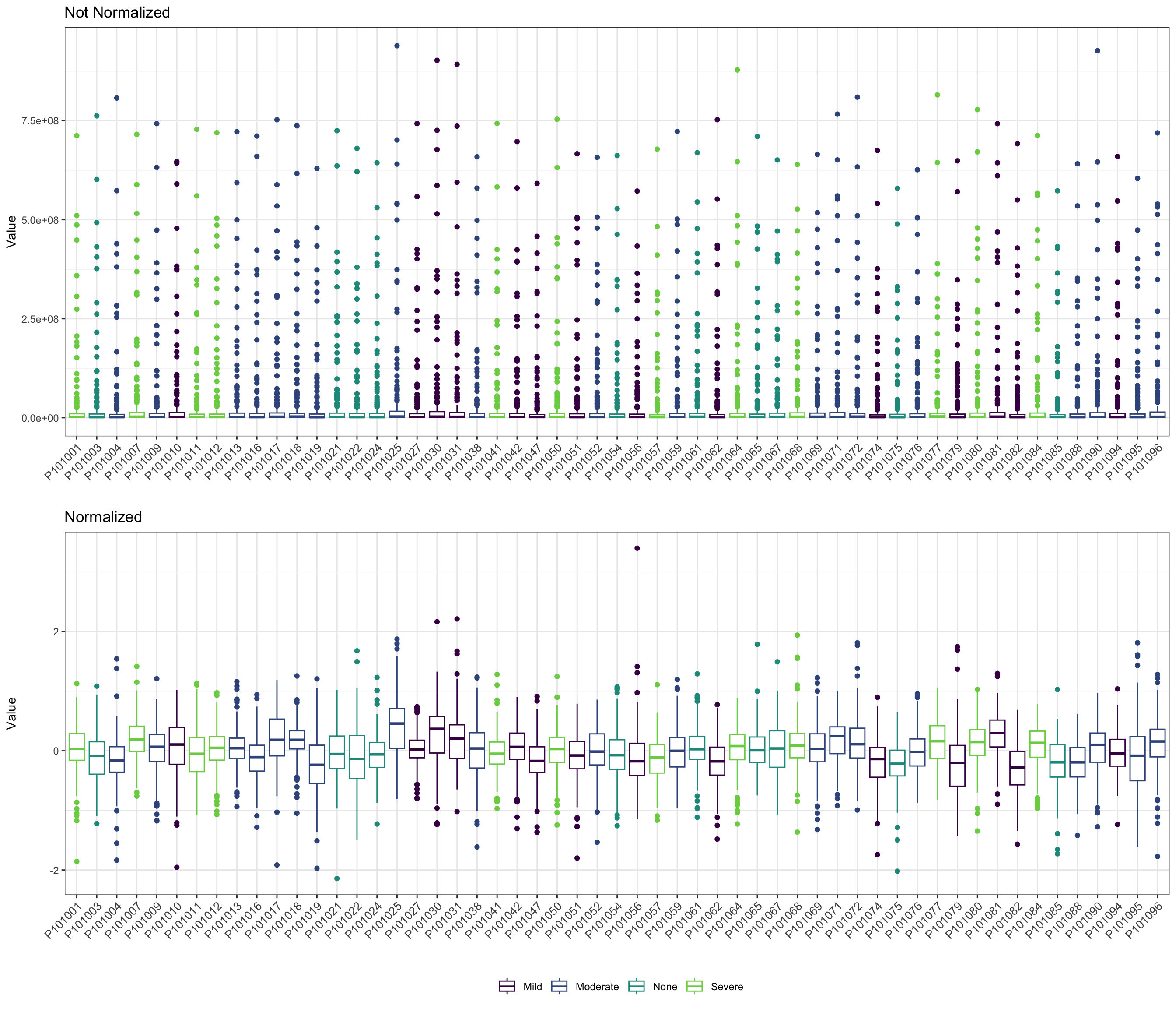
- density
pl_unnor <- PomaDensity(se_impute, group = "features") +
  ggtitle("Not Normalized") +
  theme(legend.position = "none") # data before normalization

pl_nor <- PomaDensity(se_normalize, group = "features") +
  ggtitle("Normalized") # data after normalization

cowplot::plot_grid(pl_unnor, pl_nor, ncol = 1, align = "v")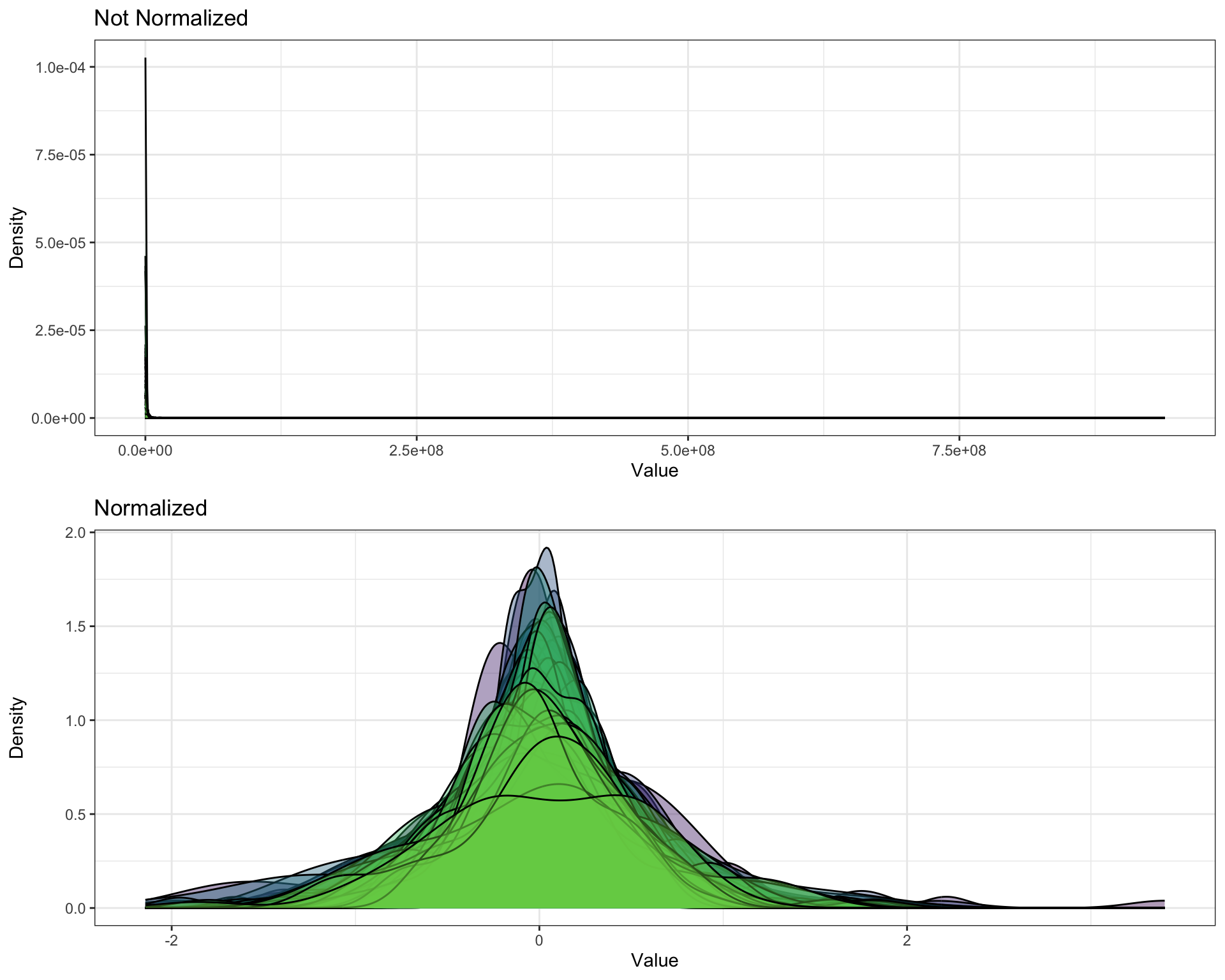
2.8 Removing outliers
Calculating the pairwise distance (distance measured by “euclidean”, “maximum”, “manhattan”, “canberra” or “minkowski”), and using 1.5 in Q3 + 1.5*IQR formula to detect outliers. More details to see ?POMA::PomaOutliers.
Caution: this step will remove samples regarded as outliers, please pay attention to your own data.
## class: SummarizedExperiment
## dim: 180 53
## metadata(0):
## assays(1): ''
## rownames(180): M_38768 M_38296 ... M_31787 M_63361
## rowData names(0):
## colnames(53): P101001 P101003 ... P101094 P101096
## colData names(5): group Gender Smoker Age AlcoholConsumption
2.9 Data distribution
get_distribution <- function(
    datset,
    Type = c("raw", "check", "filter",
             "impute", "norm_relative", "norm_log10")){

  # datset = se
  # Type = "raw"

  dat <- SummarizedExperiment::assay(datset) %>%
      data.frame() %>%
      rownames_to_column("name") %>%
      tidyr::gather(key="sample", value="value", -name)

  if (Type == "raw") {
    pl <- ggplot(dat, aes(x=value)) +
            geom_histogram(colour="black", fill="white")+
            labs(title="Distribution of Raw \n Metabolites Intensity",
                 x="Raw Intensity", y="Frequency")+
            theme_bw()
  } else if (Type == "check") {
    pl <- ggplot(dat, aes(x=value)) +
            geom_histogram(colour="black", fill="white")+
            labs(title="Distribution of check \n Metabolites Intensity",
                 x="checked Intensity", y="Frequency")+
            theme_bw()
  } else if (Type == "filter") {
    pl <- ggplot(dat, aes(x=value)) +
            geom_histogram(colour="black", fill="white")+
            labs(title="Distribution of filter\n Metabolites Intensity",
                 x="filtered Intensity", y="Frequency")+
            theme_bw()
  } else if (Type == "impute") {
    pl <- ggplot(dat, aes(x=value)) +
            geom_histogram(colour="black", fill="white")+
            labs(title="Distribution of impute\n Metabolites Intensity",
                 x="imputed Intensity", y="Frequency")+
            theme_bw()
  } else if (Type == "norm") {
    pl <- ggplot(dat, aes(x=value)) +
            geom_histogram(colour="black", fill="white")+
            labs(title="Distribution of norm\n Metabolites Intensity",
                 x="norm", y="Frequency")+
            theme_bw()
  }

  return(pl)
}

raw_pl <- get_distribution(datset=se_raw, Type="raw")
check_pl <- get_distribution(datset=se_check, Type="check")
filter_pl <- get_distribution(datset=se_filter, Type="filter")
impute_pl <- get_distribution(datset=se_impute, Type="impute")
norm_pl <- get_distribution(datset=se_normalize_v2, Type="norm")

cowplot::plot_grid(raw_pl, check_pl,
                   filter_pl, impute_pl,
                   norm_pl,
                   align = "hv", nrow = 2)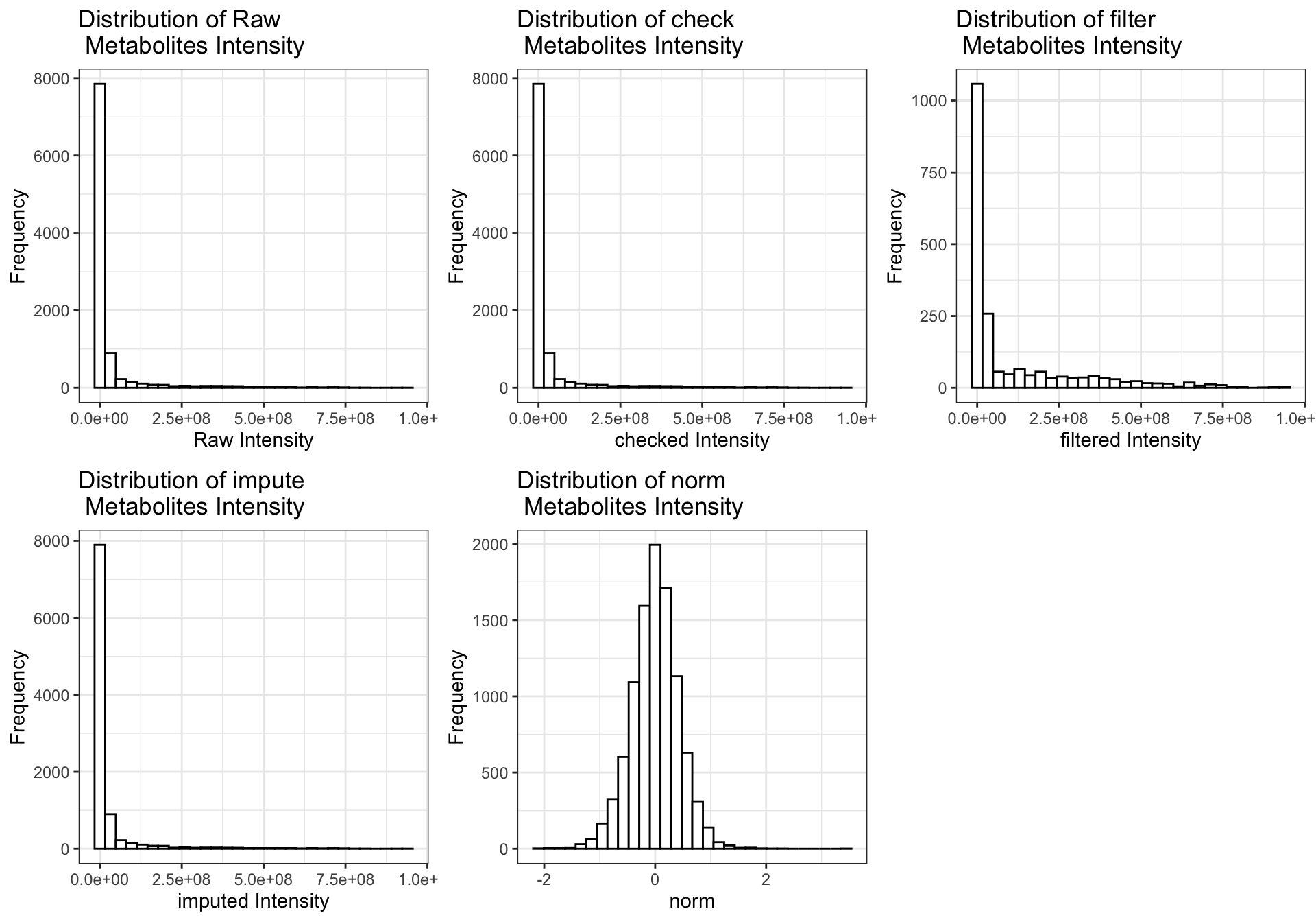
2.10 Saving datasets into RDS files
if (!dir.exists("./dataset/POMA/")) {
  dir.create("./dataset/POMA/")
}

saveRDS(ExprSet, "./dataset/POMA/ExprSet_raw.RDS", compress = TRUE)
saveRDS(se_raw, "./dataset/POMA/se_raw.RDS", compress = TRUE)
saveRDS(se_check, "./dataset/POMA/se_check.RDS", compress = TRUE)
saveRDS(se_filter, "./dataset/POMA/se_filter.RDS", compress = TRUE)
saveRDS(se_impute, "./dataset/POMA/se_impute.RDS", compress = TRUE)
saveRDS(se_normalize, "./dataset/POMA/se_normalize.RDS", compress = TRUE)
saveRDS(se_processed, "./dataset/POMA/se_processed.RDS", compress = TRUE)
2.11 Systematic Information
## ─ Session info ─────────────────────────────────────────────────────────────────────────────────────────────────────────────────────────────────────
##  setting  value
##  version  R version 4.1.3 (2022-03-10)
##  os       macOS Monterey 12.2.1
##  system   x86_64, darwin17.0
##  ui       RStudio
##  language (EN)
##  collate  en_US.UTF-8
##  ctype    en_US.UTF-8
##  tz       Asia/Shanghai
##  date     2023-12-07
##  rstudio  2023.09.0+463 Desert Sunflower (desktop)
##  pandoc   3.1.1 @ /Applications/RStudio.app/Contents/Resources/app/quarto/bin/tools/ (via rmarkdown)
##
## ─ Packages ─────────────────────────────────────────────────────────────────────────────────────────────────────────────────────────────────────────
##  package              * version    date (UTC) lib source
##  abind                  1.4-5      2016-07-21 [2] CRAN (R 4.1.0)
##  backports              1.4.1      2021-12-13 [2] CRAN (R 4.1.0)
##  base64enc              0.1-3      2015-07-28 [2] CRAN (R 4.1.0)
##  Biobase              * 2.54.0     2021-10-26 [2] Bioconductor
##  BiocGenerics         * 0.40.0     2021-10-26 [2] Bioconductor
##  BiocParallel           1.28.3     2021-12-09 [2] Bioconductor
##  bitops                 1.0-7      2021-04-24 [2] CRAN (R 4.1.0)
##  bookdown               0.34       2023-05-09 [2] CRAN (R 4.1.2)
##  broom                  1.0.5      2023-06-09 [2] CRAN (R 4.1.3)
##  bslib                  0.6.0      2023-11-21 [1] CRAN (R 4.1.3)
##  cachem                 1.0.8      2023-05-01 [2] CRAN (R 4.1.2)
##  callr                  3.7.3      2022-11-02 [2] CRAN (R 4.1.2)
##  caret                  6.0-94     2023-03-21 [2] CRAN (R 4.1.2)
##  cellranger             1.1.0      2016-07-27 [2] CRAN (R 4.1.0)
##  checkmate              2.2.0      2023-04-27 [2] CRAN (R 4.1.2)
##  circlize               0.4.15     2022-05-10 [2] CRAN (R 4.1.2)
##  class                  7.3-22     2023-05-03 [2] CRAN (R 4.1.2)
##  cli                    3.6.1      2023-03-23 [2] CRAN (R 4.1.2)
##  clue                   0.3-64     2023-01-31 [2] CRAN (R 4.1.2)
##  cluster                2.1.4      2022-08-22 [2] CRAN (R 4.1.2)
##  codetools              0.2-19     2023-02-01 [2] CRAN (R 4.1.2)
##  colorspace             2.1-0      2023-01-23 [2] CRAN (R 4.1.2)
##  ComplexHeatmap         2.10.0     2021-10-26 [2] Bioconductor
##  corpcor                1.6.10     2021-09-16 [2] CRAN (R 4.1.0)
##  cowplot                1.1.1      2020-12-30 [2] CRAN (R 4.1.0)
##  crayon                 1.5.2      2022-09-29 [2] CRAN (R 4.1.2)
##  data.table             1.14.8     2023-02-17 [2] CRAN (R 4.1.2)
##  DelayedArray           0.20.0     2021-10-26 [2] Bioconductor
##  devtools               2.4.5      2022-10-11 [2] CRAN (R 4.1.2)
##  digest                 0.6.33     2023-07-07 [1] CRAN (R 4.1.3)
##  doParallel             1.0.17     2022-02-07 [2] CRAN (R 4.1.2)
##  doRNG                  1.8.6      2023-01-16 [2] CRAN (R 4.1.2)
##  dplyr                * 1.1.2      2023-04-20 [2] CRAN (R 4.1.2)
##  e1071                  1.7-13     2023-02-01 [2] CRAN (R 4.1.2)
##  ellipse                0.4.5      2023-04-05 [2] CRAN (R 4.1.2)
##  ellipsis               0.3.2      2021-04-29 [2] CRAN (R 4.1.0)
##  evaluate               0.21       2023-05-05 [2] CRAN (R 4.1.2)
##  fansi                  1.0.4      2023-01-22 [2] CRAN (R 4.1.2)
##  farver                 2.1.1      2022-07-06 [2] CRAN (R 4.1.2)
##  fastmap                1.1.1      2023-02-24 [2] CRAN (R 4.1.2)
##  foreach                1.5.2      2022-02-02 [2] CRAN (R 4.1.2)
##  foreign                0.8-84     2022-12-06 [2] CRAN (R 4.1.2)
##  forestplot             3.1.1      2022-12-06 [2] CRAN (R 4.1.2)
##  Formula                1.2-5      2023-02-24 [2] CRAN (R 4.1.2)
##  fs                     1.6.2      2023-04-25 [2] CRAN (R 4.1.2)
##  future                 1.33.0     2023-07-01 [2] CRAN (R 4.1.3)
##  future.apply           1.11.0     2023-05-21 [2] CRAN (R 4.1.3)
##  generics               0.1.3      2022-07-05 [2] CRAN (R 4.1.2)
##  GenomeInfoDb         * 1.30.1     2022-01-30 [2] Bioconductor
##  GenomeInfoDbData       1.2.7      2022-03-09 [2] Bioconductor
##  GenomicRanges        * 1.46.1     2021-11-18 [2] Bioconductor
##  GetoptLong             1.0.5      2020-12-15 [2] CRAN (R 4.1.0)
##  ggforce                0.4.1      2022-10-04 [2] CRAN (R 4.1.2)
##  ggplot2              * 3.4.2      2023-04-03 [2] CRAN (R 4.1.2)
##  ggraph               * 2.1.0.9000 2023-07-11 [1] Github (thomasp85/ggraph@febab71)
##  ggrepel                0.9.3      2023-02-03 [2] CRAN (R 4.1.2)
##  glasso                 1.11       2019-10-01 [2] CRAN (R 4.1.0)
##  glmnet                 4.1-7      2023-03-23 [2] CRAN (R 4.1.2)
##  GlobalOptions          0.1.2      2020-06-10 [2] CRAN (R 4.1.0)
##  globals                0.16.2     2022-11-21 [2] CRAN (R 4.1.2)
##  glue                 * 1.6.2      2022-02-24 [2] CRAN (R 4.1.2)
##  Gmisc                * 3.0.2      2023-03-13 [2] CRAN (R 4.1.2)
##  gmm                    1.8        2023-06-06 [2] CRAN (R 4.1.3)
##  gmp                    0.7-1      2023-02-07 [2] CRAN (R 4.1.2)
##  gower                  1.0.1      2022-12-22 [2] CRAN (R 4.1.2)
##  graphlayouts           1.0.0      2023-05-01 [2] CRAN (R 4.1.2)
##  gridExtra              2.3        2017-09-09 [2] CRAN (R 4.1.0)
##  gtable                 0.3.3      2023-03-21 [2] CRAN (R 4.1.2)
##  hardhat                1.3.0      2023-03-30 [2] CRAN (R 4.1.2)
##  highr                  0.10       2022-12-22 [2] CRAN (R 4.1.2)
##  Hmisc                  5.1-0      2023-05-08 [2] CRAN (R 4.1.2)
##  htmlTable            * 2.4.1      2022-07-07 [2] CRAN (R 4.1.2)
##  htmltools              0.5.7      2023-11-03 [1] CRAN (R 4.1.3)
##  htmlwidgets            1.6.2      2023-03-17 [2] CRAN (R 4.1.2)
##  httpuv                 1.6.11     2023-05-11 [2] CRAN (R 4.1.3)
##  httr                   1.4.6      2023-05-08 [2] CRAN (R 4.1.2)
##  igraph                 1.5.0      2023-06-16 [1] CRAN (R 4.1.3)
##  impute                 1.68.0     2021-10-26 [2] Bioconductor
##  imputeLCMD             2.1        2022-06-10 [2] CRAN (R 4.1.2)
##  ipred                  0.9-14     2023-03-09 [2] CRAN (R 4.1.2)
##  IRanges              * 2.28.0     2021-10-26 [2] Bioconductor
##  iterators              1.0.14     2022-02-05 [2] CRAN (R 4.1.2)
##  itertools              0.1-3      2014-03-12 [2] CRAN (R 4.1.0)
##  jquerylib              0.1.4      2021-04-26 [2] CRAN (R 4.1.0)
##  jsonlite               1.8.7      2023-06-29 [2] CRAN (R 4.1.3)
##  knitr                  1.43       2023-05-25 [2] CRAN (R 4.1.3)
##  labeling               0.4.2      2020-10-20 [2] CRAN (R 4.1.0)
##  later                  1.3.1      2023-05-02 [2] CRAN (R 4.1.2)
##  lattice                0.21-8     2023-04-05 [2] CRAN (R 4.1.2)
##  lava                   1.7.2.1    2023-02-27 [2] CRAN (R 4.1.2)
##  lazyeval               0.2.2      2019-03-15 [2] CRAN (R 4.1.0)
##  lifecycle              1.0.3      2022-10-07 [2] CRAN (R 4.1.2)
##  limma                  3.50.3     2022-04-07 [2] Bioconductor
##  listenv                0.9.0      2022-12-16 [2] CRAN (R 4.1.2)
##  lubridate              1.9.2      2023-02-10 [2] CRAN (R 4.1.2)
##  magrittr             * 2.0.3      2022-03-30 [2] CRAN (R 4.1.2)
##  MASS                   7.3-60     2023-05-04 [2] CRAN (R 4.1.2)
##  Matrix                 1.6-0      2023-07-08 [2] CRAN (R 4.1.3)
##  MatrixGenerics       * 1.6.0      2021-10-26 [2] Bioconductor
##  matrixStats          * 1.0.0      2023-06-02 [2] CRAN (R 4.1.3)
##  memoise                2.0.1      2021-11-26 [2] CRAN (R 4.1.0)
##  mgcv                   1.8-42     2023-03-02 [2] CRAN (R 4.1.2)
##  mime                   0.12       2021-09-28 [2] CRAN (R 4.1.0)
##  miniUI                 0.1.1.1    2018-05-18 [2] CRAN (R 4.1.0)
##  missForest             1.5        2022-04-14 [2] CRAN (R 4.1.2)
##  mixOmics               6.18.1     2021-11-18 [2] Bioconductor (R 4.1.2)
##  ModelMetrics           1.2.2.2    2020-03-17 [2] CRAN (R 4.1.0)
##  munsell                0.5.0      2018-06-12 [2] CRAN (R 4.1.0)
##  mvtnorm                1.2-2      2023-06-08 [2] CRAN (R 4.1.3)
##  nlme                   3.1-162    2023-01-31 [2] CRAN (R 4.1.2)
##  nnet                   7.3-19     2023-05-03 [2] CRAN (R 4.1.2)
##  norm                   1.0-11.1   2023-06-18 [2] CRAN (R 4.1.3)
##  parallelly             1.36.0     2023-05-26 [2] CRAN (R 4.1.3)
##  pcaMethods             1.86.0     2021-10-26 [2] Bioconductor
##  permute                0.9-7      2022-01-27 [2] CRAN (R 4.1.2)
##  pillar                 1.9.0      2023-03-22 [2] CRAN (R 4.1.2)
##  pkgbuild               1.4.2      2023-06-26 [2] CRAN (R 4.1.3)
##  pkgconfig              2.0.3      2019-09-22 [2] CRAN (R 4.1.0)
##  pkgload                1.3.2.1    2023-07-08 [2] CRAN (R 4.1.3)
##  plotly               * 4.10.2     2023-06-03 [2] CRAN (R 4.1.3)
##  plyr                   1.8.8      2022-11-11 [2] CRAN (R 4.1.2)
##  png                    0.1-8      2022-11-29 [2] CRAN (R 4.1.2)
##  polyclip               1.10-4     2022-10-20 [2] CRAN (R 4.1.2)
##  POMA                 * 1.7.2      2022-07-26 [2] Github (pcastellanoescuder/POMA@bc8a972)
##  preprocessCore         1.56.0     2021-10-26 [2] Bioconductor
##  prettyunits            1.1.1      2020-01-24 [2] CRAN (R 4.1.0)
##  pROC                   1.18.4     2023-07-06 [2] CRAN (R 4.1.3)
##  processx               3.8.2      2023-06-30 [2] CRAN (R 4.1.3)
##  prodlim                2023.03.31 2023-04-02 [2] CRAN (R 4.1.2)
##  profvis                0.3.8      2023-05-02 [2] CRAN (R 4.1.2)
##  promises               1.2.0.1    2021-02-11 [2] CRAN (R 4.1.0)
##  proxy                  0.4-27     2022-06-09 [2] CRAN (R 4.1.2)
##  ps                     1.7.5      2023-04-18 [2] CRAN (R 4.1.2)
##  purrr                  1.0.1      2023-01-10 [2] CRAN (R 4.1.2)
##  R6                     2.5.1      2021-08-19 [2] CRAN (R 4.1.0)
##  randomForest           4.7-1.1    2022-05-23 [2] CRAN (R 4.1.2)
##  RankProd               3.20.0     2021-10-26 [2] Bioconductor
##  rARPACK                0.11-0     2016-03-10 [2] CRAN (R 4.1.0)
##  RColorBrewer           1.1-3      2022-04-03 [2] CRAN (R 4.1.2)
##  Rcpp                 * 1.0.11     2023-07-06 [1] CRAN (R 4.1.3)
##  RCurl                  1.98-1.12  2023-03-27 [2] CRAN (R 4.1.2)
##  readxl               * 1.4.3      2023-07-06 [2] CRAN (R 4.1.3)
##  recipes                1.0.6      2023-04-25 [2] CRAN (R 4.1.2)
##  remotes                2.4.2      2021-11-30 [2] CRAN (R 4.1.0)
##  reshape2               1.4.4      2020-04-09 [2] CRAN (R 4.1.0)
##  rjson                  0.2.21     2022-01-09 [2] CRAN (R 4.1.2)
##  rlang                  1.1.1      2023-04-28 [1] CRAN (R 4.1.2)
##  rmarkdown              2.23       2023-07-01 [2] CRAN (R 4.1.3)
##  Rmpfr                  0.9-2      2023-04-22 [2] CRAN (R 4.1.2)
##  rngtools               1.5.2      2021-09-20 [2] CRAN (R 4.1.0)
##  ropls                  1.26.4     2022-01-11 [2] Bioconductor
##  rpart                  4.1.19     2022-10-21 [2] CRAN (R 4.1.2)
##  RSpectra               0.16-1     2022-04-24 [2] CRAN (R 4.1.2)
##  rstudioapi             0.15.0     2023-07-07 [2] CRAN (R 4.1.3)
##  S4Vectors            * 0.32.4     2022-03-29 [2] Bioconductor
##  sandwich               3.0-2      2022-06-15 [2] CRAN (R 4.1.2)
##  sass                   0.4.6      2023-05-03 [2] CRAN (R 4.1.2)
##  scales                 1.2.1      2022-08-20 [2] CRAN (R 4.1.2)
##  sessioninfo            1.2.2      2021-12-06 [2] CRAN (R 4.1.0)
##  shape                  1.4.6      2021-05-19 [2] CRAN (R 4.1.0)
##  shiny                  1.7.4.1    2023-07-06 [2] CRAN (R 4.1.3)
##  stringi                1.7.12     2023-01-11 [2] CRAN (R 4.1.2)
##  stringr                1.5.0      2022-12-02 [2] CRAN (R 4.1.2)
##  SummarizedExperiment * 1.24.0     2021-10-26 [2] Bioconductor
##  survival               3.5-5      2023-03-12 [2] CRAN (R 4.1.2)
##  tibble               * 3.2.1      2023-03-20 [2] CRAN (R 4.1.2)
##  tidygraph              1.2.3      2023-02-01 [2] CRAN (R 4.1.2)
##  tidyr                  1.3.0      2023-01-24 [2] CRAN (R 4.1.2)
##  tidyselect             1.2.0      2022-10-10 [2] CRAN (R 4.1.2)
##  timechange             0.2.0      2023-01-11 [2] CRAN (R 4.1.2)
##  timeDate               4022.108   2023-01-07 [2] CRAN (R 4.1.2)
##  tmvtnorm               1.5        2022-03-22 [2] CRAN (R 4.1.2)
##  tweenr                 2.0.2      2022-09-06 [2] CRAN (R 4.1.2)
##  urlchecker             1.0.1      2021-11-30 [2] CRAN (R 4.1.0)
##  usethis                2.2.2      2023-07-06 [2] CRAN (R 4.1.3)
##  utf8                   1.2.3      2023-01-31 [2] CRAN (R 4.1.2)
##  vctrs                  0.6.3      2023-06-14 [1] CRAN (R 4.1.3)
##  vegan                  2.6-4      2022-10-11 [2] CRAN (R 4.1.2)
##  viridis                0.6.3      2023-05-03 [2] CRAN (R 4.1.2)
##  viridisLite            0.4.2      2023-05-02 [2] CRAN (R 4.1.2)
##  withr                  2.5.0      2022-03-03 [2] CRAN (R 4.1.2)
##  xfun                   0.40       2023-08-09 [1] CRAN (R 4.1.3)
##  XML                    3.99-0.14  2023-03-19 [2] CRAN (R 4.1.2)
##  xtable                 1.8-4      2019-04-21 [2] CRAN (R 4.1.0)
##  XVector                0.34.0     2021-10-26 [2] Bioconductor
##  yaml                   2.3.7      2023-01-23 [2] CRAN (R 4.1.2)
##  zlibbioc               1.40.0     2021-10-26 [2] Bioconductor
##  zoo                    1.8-12     2023-04-13 [2] CRAN (R 4.1.2)
##
##  [1] /Users/zouhua/Library/R/x86_64/4.1/library
##  [2] /Library/Frameworks/R.framework/Versions/4.1/Resources/library
##
## ────────────────────────────────────────────────────────────────────────────────────────────────────────────────────────────────────────────────────