Chapter 9 Network Analysis
Estimating microbial association networks from high-throughput sequencing data is a common exploratory data analysis approach aiming at understanding the complex interplay of microbial communities in their natural habitat. Statistical network estimation workflows comprise several analysis steps, including methods for zero handling, data normalization and computing microbial associations. Since microbial interactions are likely to change between conditions, e.g. between healthy individuals and patients, identifying network differences between groups is often an integral secondary analysis step.
NetCoMi (Network Construction and Comparison for Microbiome Data) (Peschel et al. 2021) provides functionality for constructing, analyzing, and comparing networks suitable for the application on microbial compositional data.
The following information is from NetCoMi github.
Association measures:
- Pearson coefficient
(
cor()fromstatspackage) - Spearman coefficient
(
cor()fromstatspackage) - Biweight Midcorrelation
bicor()fromWGCNApackage - SparCC
(
sparcc()fromSpiecEasipackage) - CCLasso (R code on GitHub)
- CCREPE
(
ccrepepackage) - SpiecEasi (
SpiecEasipackage) - SPRING (
SPRINGpackage) - gCoda (R code on GitHub)
- propr
(
proprpackage)
Dissimilarity measures:
- Euclidean distance
(
vegdist()fromveganpackage) - Bray-Curtis dissimilarity
(
vegdist()fromveganpackage) - Kullback-Leibler divergence (KLD)
(
KLD()fromLaplacesDemonpackage) - Jeffrey divergence (own code using
KLD()fromLaplacesDemonpackage) - Jensen-Shannon divergence (own code using
KLD()fromLaplacesDemonpackage) - Compositional KLD (own implementation following [Martín-Fernández et al., 1999])
- Aitchison distance
(
vegdist()andclr()fromSpiecEasipackage)
Methods for zero replacement:
- Adding a predefined pseudo count
- Multiplicative replacement
(
multReplfromzCompositionspackage) - Modified EM alr-algorithm
(
lrEMfromzCompositionspackage) - Bayesian-multiplicative replacement
(
cmultReplfromzCompositionspackage)
Normalization methods:
- Total Sum Scaling (TSS) (own implementation)
- Cumulative Sum Scaling (CSS) (
cumNormMatfrommetagenomeSeqpackage) - Common Sum Scaling (COM) (own implementation)
- Rarefying (
rrarefyfromveganpackage) - Variance Stabilizing Transformation (VST)
(
varianceStabilizingTransformationfromDESeq2package) - Centered log-ratio (clr) transformation
(
clr()fromSpiecEasipackage))
TSS, CSS, COM, VST, and the clr transformation are described in [Badri et al., 2020].
Loading packages
9.1 Importing data
dada2_ps_remove_BRS <- get_GroupPhyloseq(
                         ps = dada2_ps,
                         group = "Group",
                         group_names = "QC",
                         discard = TRUE)

dada2_ps_rare <- norm_rarefy(object = dada2_ps_remove_BRS,
                             size = 51181)

dada2_ps_rare_genus <- summarize_taxa(ps = dada2_ps_rare,
                                 taxa_level = "Genus")

dada2_ps_rare_genus_filter <- run_filter(ps = dada2_ps_rare_genus,
                                         cutoff = 10,
                                         unclass = TRUE)

dada2_ps_rare_genus_filter
## phyloseq-class experiment-level object
## otu_table() OTU Table: [ 98 taxa and 23 samples ]
## sample_data() Sample Data: [ 23 samples by 1 sample variables ]
## tax_table() Taxonomy Table: [ 98 taxa by 6 taxonomic ranks ]9.2 Single network with Pearson correlation as association measure
Since Pearson correlations may lead to compositional effects when applied to sequencing data, we use the clr transformation as normalization method. Zero treatment is necessary in this case.
A threshold of 0.3 is used as sparsification method, so that only OTUs with an absolute correlation greater than or equal to 0.3 are connected.
9.2.2 Analyzing the constructed network
NetCoMi’s netAnalyze() function is used for analyzing the constructed network(s).
props_single <- netAnalyze(net_single, clustMethod = "cluster_fast_greedy")

summary(props_single, numbNodes = 5L)
##
## Component sizes
## ```````````````
## size: 7 3 2 1
## #: 1 3 5 72
## ______________________________
## Global network properties
## `````````````````````````
## Largest connected component (LCC):
##
## Relative LCC size 0.07143
## Clustering coefficient 0.54906
## Modularity 0.30469
## Positive edge percentage 50.00000
## Edge density 0.38095
## Natural connectivity 0.24942
## Vertex connectivity 1.00000
## Edge connectivity 1.00000
## Average dissimilarity* 0.85842
## Average path length** 1.21987
##
## Whole network:
##
## Number of components 81.00000
## Clustering coefficient 0.36604
## Modularity 0.77562
## Positive edge percentage 57.89474
## Edge density 0.00400
## Natural connectivity 0.01124
##
## *Dissimilarity = 1 - edge weight
## **Path length: Units with average dissimilarity
##
## ______________________________
## Clusters
## - In the whole network
## - Algorithm: cluster_fast_greedy
## ````````````````````````````````
##
## name: 0 1 2 3 4 5 6 7 8 9
## #: 72 7 3 3 3 2 2 2 2 2
##
## ______________________________
## Hubs
## - In alphabetical/numerical order
## - Based on empirical quantiles of centralities
## ```````````````````````````````````````````````
## g__Catenibacterium
## g__Coprococcus_2
## g__Holdemanella
## g__Prevotella_9
## g__Senegalimassilia
##
## ______________________________
## Centrality measures
## - In decreasing order
## - Centrality of disconnected components is zero
## ````````````````````````````````````````````````
## Degree (normalized):
##
## g__Catenibacterium 0.04124
## g__Senegalimassilia 0.03093
## g__Butyricimonas 0.02062
## g__Coprococcus_2 0.02062
## g__Odoribacter 0.02062
##
## Betweenness centrality (normalized):
##
## g__Catenibacterium 0.60000
## g__Coprococcus_2 0.53333
## g__Prevotella_9 0.33333
## g__Senegalimassilia 0.06667
## g__Acidaminococcus 0.00000
##
## Closeness centrality (normalized):
##
## g__Catenibacterium 1.63694
## g__Coprococcus_2 1.48298
## g__Senegalimassilia 1.41360
## g__Prevotella_9 1.39706
## g__Holdemanella 1.05263
##
## Eigenvector centrality (normalized):
##
## g__Coprococcus_2 1.00000
## g__Catenibacterium 0.95940
## g__Prevotella_9 0.85306
## g__Senegalimassilia 0.63574
## g__Holdemanella 0.491339.2.3 Visualizing the network
- primary plot
plot(props_single,
     nodeColor = "cluster",
     nodeSize = "eigenvector",
     title1 = "Network on 16s with Pearson correlations",
     showTitle = TRUE,
     labelLength = 10,
     cexTitle = 1.5)

legend(0.7, 1.1, cex = 1, title = "estimated correlation:",
       legend = c("+","-"), lty = 1, lwd = 3, col = c("#009900","red"),
       bty = "n", horiz = TRUE)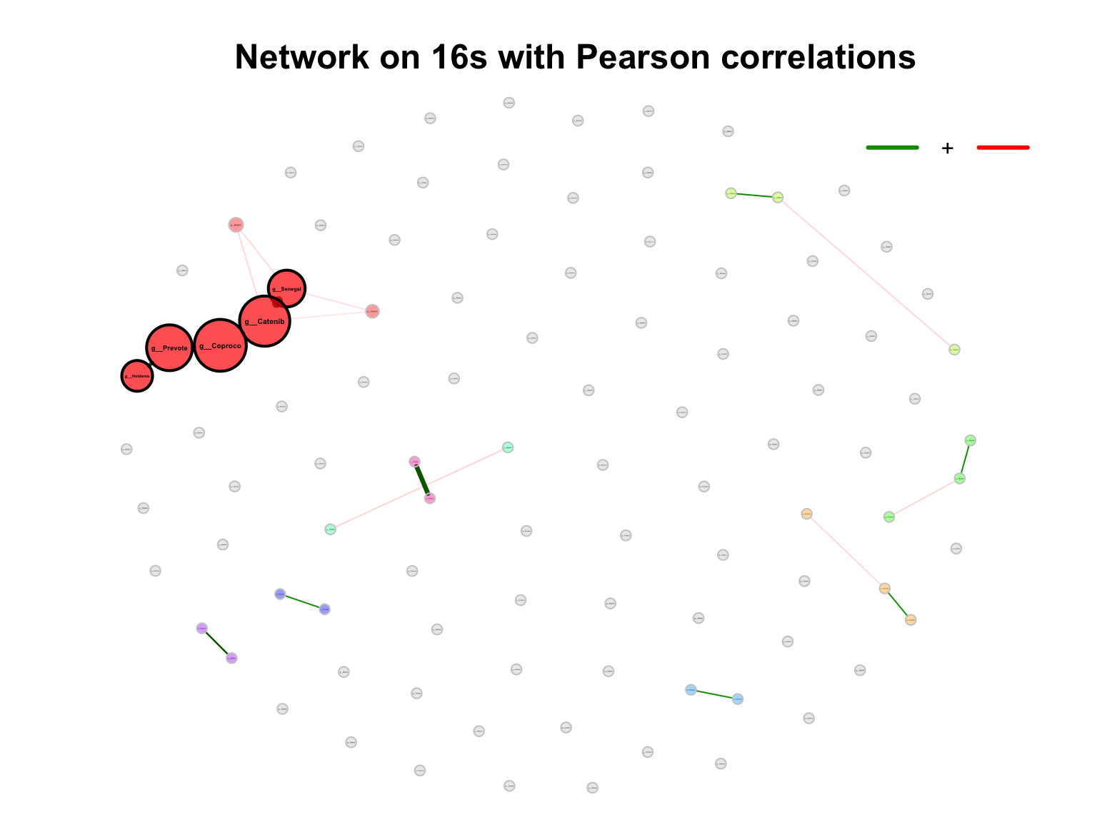
Figure 9.1: Network on 16s with Pearson correlations
improve the visualization by changing the following arguments:
repulsion = 0.8: Place the nodes further apartrmSingles = TRUE: Single nodes are removedlabelScale = FALSEandcexLabels = 1.6: All labels have equal size and are enlarged to improve readability of small node’s labelsnodeSizeSpread = 3(default is 4): Node sizes are more similar if the value is decreased. This argument (in combination withcexNodes) is useful to enlarge small nodes while keeping the size of big nodes.
plot(props_single,
     nodeColor = "cluster",
     nodeSize = "eigenvector",
     labelLength = 40,
     repulsion = 0.8,
     rmSingles = TRUE,
     labelScale = FALSE,
     cexLabels = 1,
     nodeSizeSpread = 3,
     cexNodes = 2,
     title1 = "Network on metabolomics with Pearson correlations",
     showTitle = TRUE,
     cexTitle = 1.5)

legend(0.7, 1.1, cex = 1.2, title = "estimated correlation:",
       legend = c("+","-"), lty = 1, lwd = 3, col = c("#009900","red"),
       bty = "n", horiz = TRUE)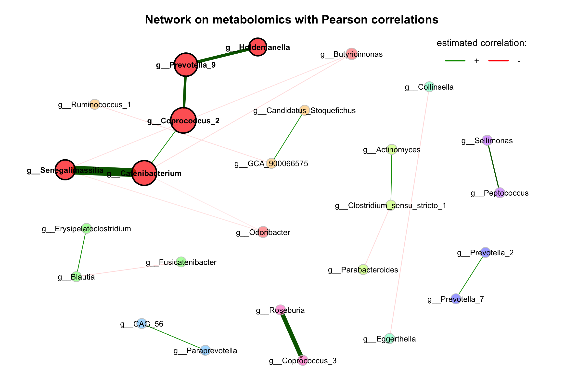
Figure 9.2: Network on 16s with Pearson correlations
- Network on genus level with Pearson correlations
set.seed(123)

graph <- igraph::graph_from_adjacency_matrix(net_single$adjaMat1, weighted = TRUE)
lay_fr <- igraph::layout_with_fr(graph)
rownames(lay_fr) <- rownames(net_single$adjaMat1)

plot(props_single,
     layout = "layout_with_fr",
     shortenLabels = "simple",
     labelLength = 30,
     charToRm = "g__",
     labelScale = FALSE,
     rmSingles = TRUE,
     nodeSize = "clr",
     nodeColor = "cluster",
     hubBorderCol = "darkgray",
     cexNodes = 2,
     cexLabels = 1.5,
     cexHubLabels = 2,
     title1 = "Network on genus level with Pearson correlations",
     showTitle = TRUE,
     cexTitle = 2.3)

legend(0.7, 1.1, cex = 2.2, title = "estimated correlation:",
       legend = c("+","-"), lty = 1, lwd = 3, col = c("#009900","red"),
       bty = "n", horiz = TRUE)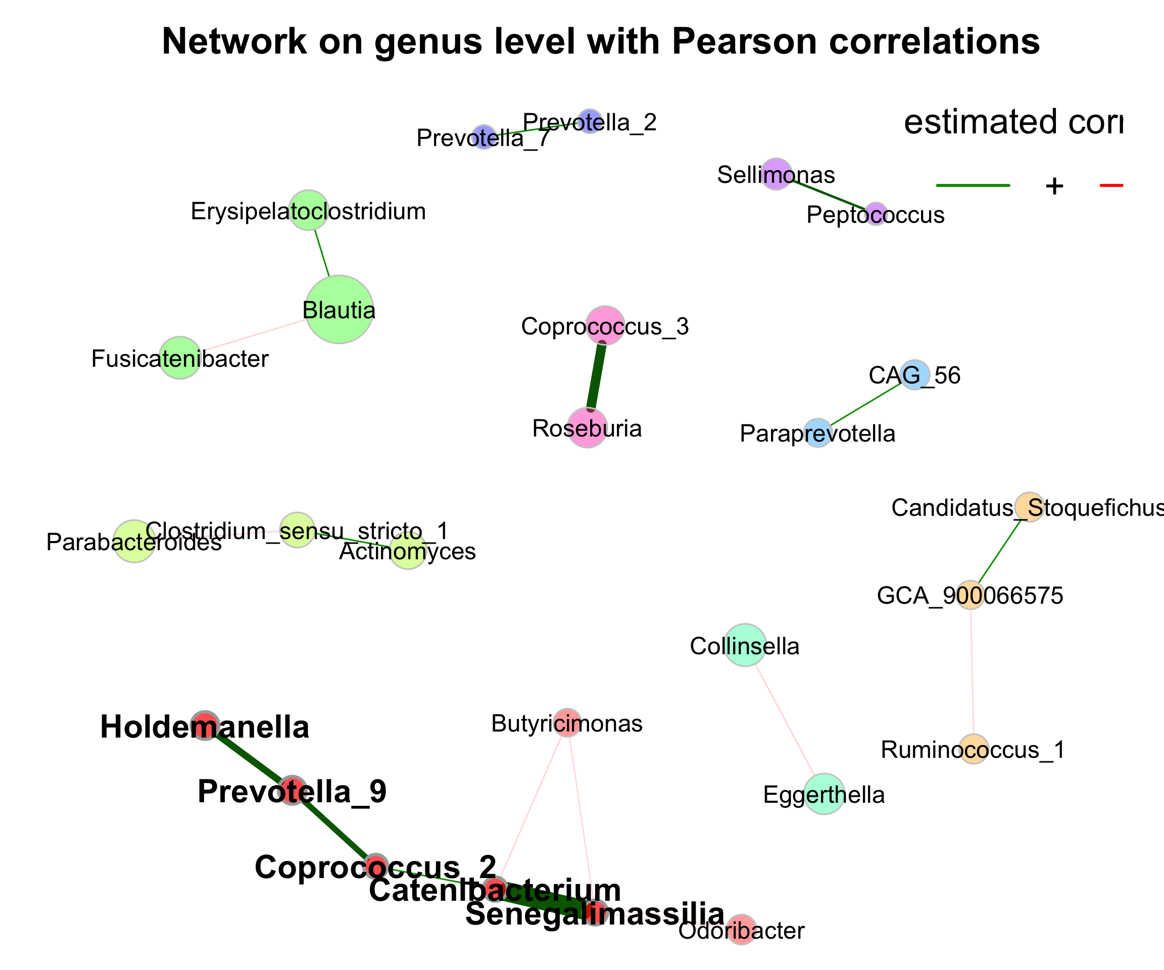
Figure 9.3: Network on 16s with Pearson correlations (Genus)
Let’s check whether the largest nodes are actually those with highest column sums in the matrix with normalized counts returned by netConstruct().
##           g__Blautia   g__Bifidobacterium       g__Bacteroides  g__Faecalibacterium     g__Streptococcus      g__Anaerostipes
##            112.41527             96.49623             82.74483             52.85493             52.20123             39.91639
##       g__Collinsella g__Lachnoclostridium      g__Agathobacter             g__Dorea
## 32.91418 31.04379 29.89418 29.32480- Network on genus level with Pearson correlations with phylum annotation
# Get phyla names from the taxonomic table created before
taxatab <- dada2_ps_rare_genus_filter@tax_table %>%
  data.frame()
phyla <- as.factor(gsub("p__", "", taxatab[, "Phylum"]))
names(phyla) <- taxatab$Genus

# Define phylum colors
phylcol <- c("cyan", "blue3", "red", "lawngreen", "yellow", "deeppink", "grey", "green")

plot(props_single,
     layout = "spring",
     repulsion = 0.84,
     shortenLabels = "none",
     charToRm = "g__",
     labelLength = 30,
     labelScale = FALSE,
     rmSingles = TRUE,
     nodeSize = "clr",
     nodeSizeSpread = 4,
     nodeColor = "feature",
     featVecCol = phyla,
     colorVec =  phylcol,
     posCol = "darkturquoise",
     negCol = "orange",
     edgeTranspLow = 0,
     edgeTranspHigh = 40,
     cexNodes = 2,
     cexLabels = 2,
     cexHubLabels = 2.5,
     title1 = "Network on genus level with Pearson correlations",
     showTitle = TRUE,
     cexTitle = 2.3)

# Colors used in the legend should be equally transparent as in the plot
phylcol_transp <- NetCoMi:::colToTransp(phylcol, 60)

legend(-1.2, 1.2, cex = 2, pt.cex = 2.5, title = "Phylum:",
       legend=levels(phyla), col = phylcol_transp, bty = "n", pch = 16)

legend(0.7, 1.1, cex = 2.2, title = "estimated correlation:",
       legend = c("+","-"), lty = 1, lwd = 3, col = c("darkturquoise","orange"),
       bty = "n", horiz = TRUE)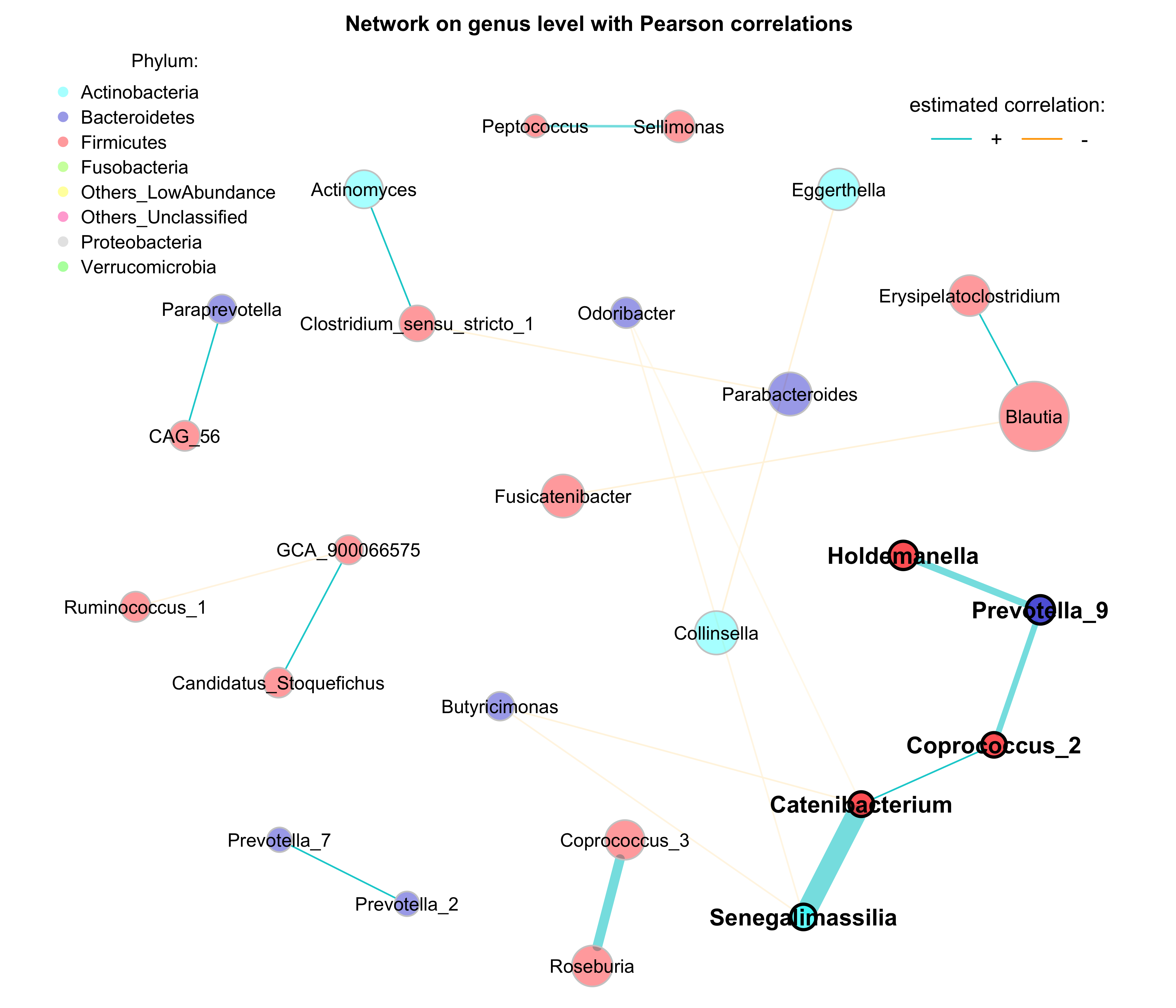
Figure 9.4: Network on 16s with Pearson correlations (Annotation)
9.3 Single network with sparcc correlation as association measure
Only the 100 features with highest variance are selected.
Only samples with a total number of reads of at least 1000 included.
9.3.1 Building network model
net_single2 <- netConstruct(dada2_ps_rare_genus_filter,
                           measure = "sparcc",
                           measurePar = list(iter = 20,
                                             inner_iter = 10,
                                             th = 0.1),
                           filtTax = "highestVar",
                           filtTaxPar = list(highestVar = 100),
                           filtSamp = "totalReads",
                           filtSampPar = list(totalReads = 100),
                           verbose = 3,
                           seed = 123)
## Data filtering ...## 98 taxa and 23 samples remaining.##
## Calculate 'sparcc' associations ... Done.
##
## Sparsify associations via 't-test' ...
## Adjust for multiple testing via 'adaptBH' ...
## Proportion of true null hypotheses: 0.87
## Done.
## Done.9.3.2 Analyzing the constructed network
NetCoMi’s netAnalyze() function is used for analyzing the constructed network(s).
props_single2 <- netAnalyze(net_single2, clustMethod = "cluster_fast_greedy")

summary(props_single2, numbNodes = 5L)
##
## Component sizes
## ```````````````
## size: 2 1
## #: 5 88
## ______________________________
## Global network properties
## `````````````````````````
## Largest connected component (LCC):
##
## Relative LCC size 0.02041
## Clustering coefficient 0.00000
## Modularity 0.00000
## Positive edge percentage 100.00000
## Edge density 1.00000
## Natural connectivity 0.93633
## Vertex connectivity 1.00000
## Edge connectivity 1.00000
## Average dissimilarity* 0.30602
## Average path length** 1.00000
##
## Whole network:
##
## Number of components 93.00000
## Clustering coefficient 0.00000
## Modularity 0.80000
## Positive edge percentage 80.00000
## Edge density 0.00105
## Natural connectivity 0.01092
##
## *Dissimilarity = 1 - edge weight
## **Path length: Units with average dissimilarity
##
## ______________________________
## Clusters
## - In the whole network
## - Algorithm: cluster_fast_greedy
## ````````````````````````````````
##
## name: 0 1 2 3 4 5
## #: 88 2 2 2 2 2
##
## ______________________________
## Hubs
## - In alphabetical/numerical order
## - Based on empirical quantiles of centralities
## ```````````````````````````````````````````````
## g__Blautia
## g__Erysipelatoclostridium
##
## ______________________________
## Centrality measures
## - In decreasing order
## - Centrality of disconnected components is zero
## ````````````````````````````````````````````````
## Degree (normalized):
##
## g__Blautia 0.01031
## g__Erysipelatoclostridium 0.01031
## g__Acidaminococcus 0.00000
## g__Actinomyces 0.00000
## g__Adlercreutzia 0.00000
##
## Betweenness centrality (normalized):
##
## g__Acidaminococcus 0
## g__Actinomyces 0
## g__Adlercreutzia 0
## g__Agathobacter 0
## g__Akkermansia 0
##
## Closeness centrality (normalized):
##
## g__Blautia 1
## g__Erysipelatoclostridium 1
## g__Acidaminococcus 0
## g__Actinomyces 0
## g__Adlercreutzia 0
##
## Eigenvector centrality (normalized):
##
## g__Blautia 1
## g__Erysipelatoclostridium 1
## g__Acidaminococcus 0
## g__Actinomyces 0
## g__Adlercreutzia 09.3.2.1 Visualizing the network
plot(props_single2,
     layout = "spring",
     repulsion = 0.84,
     shortenLabels = "none",
     charToRm = "g__",
     labelLength = 30,
     labelScale = FALSE,
     rmSingles = TRUE,
     nodeSize = "clr",
     nodeSizeSpread = 4,
     nodeColor = "feature",
     featVecCol = phyla,
     colorVec =  phylcol,
     posCol = "darkturquoise",
     negCol = "orange",
     edgeTranspLow = 0,
     edgeTranspHigh = 40,
     cexNodes = 2,
     cexLabels = 2,
     cexHubLabels = 2.5,
     title1 = "Network on genus level with Pearson correlations",
     showTitle = TRUE,
     cexTitle = 2.3)

# Colors used in the legend should be equally transparent as in the plot
phylcol_transp <- NetCoMi:::colToTransp(phylcol, 60)

legend(-1.2, 1.2, cex = 2, pt.cex = 2.5, title = "Phylum:",
       legend=levels(phyla), col = phylcol_transp, bty = "n", pch = 16)

legend(0.7, 1.1, cex = 2.2, title = "estimated correlation:",
       legend = c("+","-"), lty = 1, lwd = 3, col = c("darkturquoise","orange"),
       bty = "n", horiz = TRUE)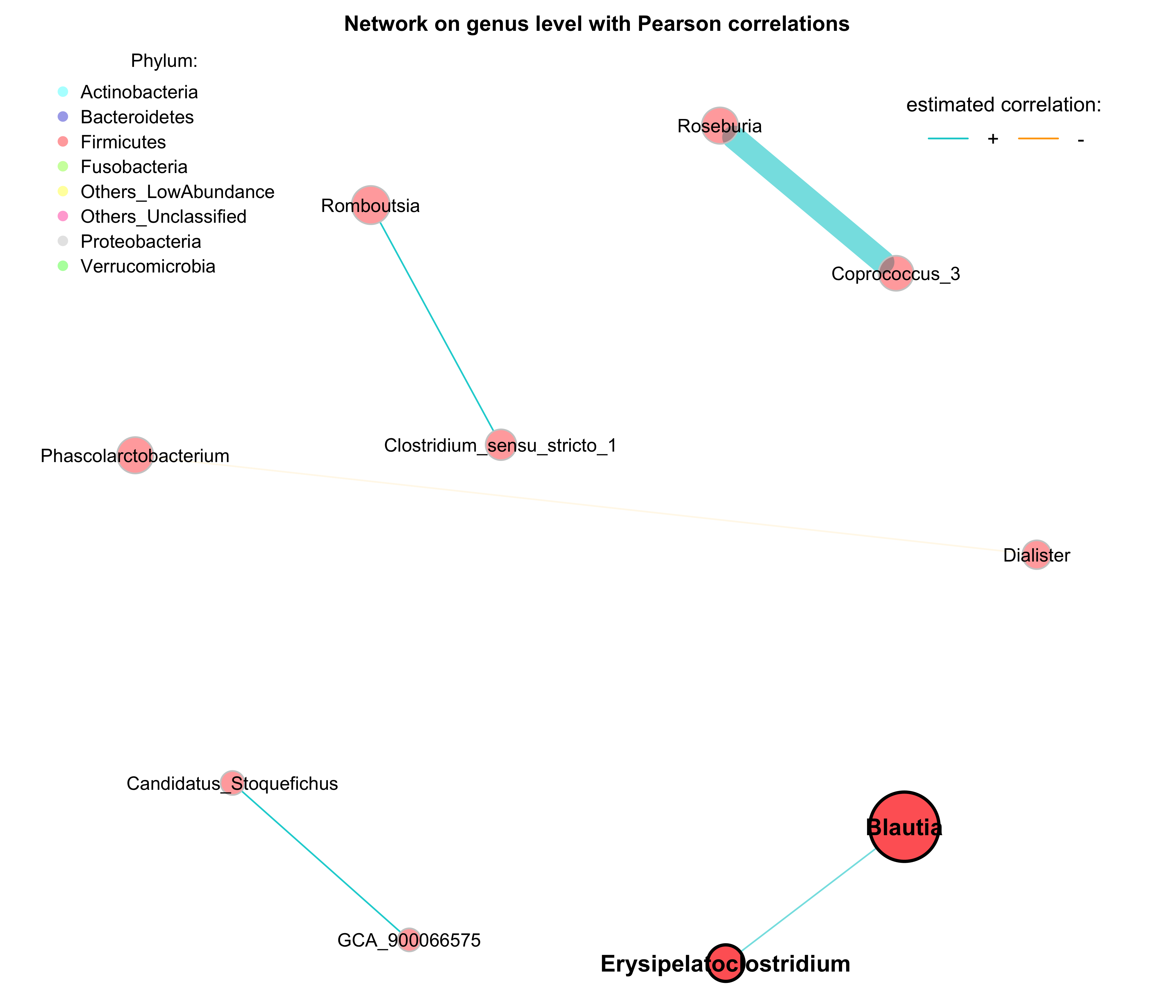
Figure 9.5: Network on metabolomics with sparcc associations
9.4 Dissimilarity-based Networks
If a dissimilarity measure is used for network construction, nodes are subjects instead of OTUs. The estimated dissimilarities are transformed into similarities, which are used as edge weights so that subjects with a similar microbial composition are placed close together in the network plot.
We construct a single network using Aitchison’s distance being suitable for the application on compositional data.
Since the Aitchison distance is based on the clr-transformation, zeros in the data need to be replaced.
The network is sparsified using the k-nearest neighbor (knn) algorithm.
9.4.1 Building network module
net_aitchison <- netConstruct(dada2_ps_rare_genus_filter,
                              measure = "aitchison",
                              zeroMethod = "multRepl",
                              sparsMethod = "knn",
                              kNeighbor = 3,
                              verbose = 3)
## Infos about changed arguments:## Counts normalized to fractions for measure 'aitchison'.## 98 taxa and 23 samples remaining.##
## Zero treatment:## Execute multRepl() ...## Warning in (function (X, label = NULL, dl = NULL, frac = 0.65, imp.missing = FALSE, : Column(s) containing more than 80% zeros/unobserved values were found (check it out using zPatterns).
## (You can use the z.warning argument to modify the warning threshold).## Done.
##
## Normalization:
## Counts normalized by total sum scaling.
##
## Calculate 'aitchison' dissimilarities ... Done.
##
## Sparsify dissimilarities via 'knn' ... Done.9.4.2 Analyzing the constructed network
NetCoMi’s netAnalyze() function is used for analyzing the constructed network(s).
props_aitchison <- netAnalyze(net_aitchison,
                              clustMethod = "hierarchical",
                              clustPar = list(method = "average", k = 3),
                              hubPar = "eigenvector")

summary(props_aitchison, numbNodes = 5L)
##
## Component sizes
## ```````````````
## size: 23
## #: 1
## ______________________________
## Global network properties
## `````````````````````````
##
## Number of components 1.00000
## Clustering coefficient 0.38932
## Modularity 0.38909
## Positive edge percentage 100.00000
## Edge density 0.18577
## Natural connectivity 0.11078
## Vertex connectivity 2.00000
## Edge connectivity 3.00000
## Average dissimilarity* 0.86903
## Average path length** 0.81512
##
## *Dissimilarity = 1 - edge weight
## **Path length: Units with average dissimilarity
##
## ______________________________
## Clusters
## - In the whole network
## - Algorithm: hierarchical
## `````````````````````````
##
## name: 1 2 3
## #: 3 9 11
##
## ______________________________
## Hubs
## - In alphabetical/numerical order
## - Based on empirical quantiles of centralities
## ```````````````````````````````````````````````
## S6035
## S6063
##
## ______________________________
## Centrality measures
## - In decreasing order
## - Computed for the complete network
## ````````````````````````````````````
## Degree (normalized):
##
## S6055 0.31818
## S6063 0.31818
## S6032 0.27273
## S6035 0.27273
## S6059 0.22727
##
## Betweenness centrality (normalized):
##
## S6046 0.31169
## S6055 0.30736
## S6035 0.29437
## S6063 0.28571
## S6032 0.14719
##
## Closeness centrality (normalized):
##
## S6050 2.77533
## S6040 2.76253
## S6055 2.61632
## S6035 2.55776
## S6046 2.53153
##
## Eigenvector centrality (normalized):
##
## S6063 1.00000
## S6035 0.86425
## S6032 0.84981
## S6068 0.73759
## S6037 0.621679.4.3 Visualizing the network
- primary plot
plot(props_aitchison,
     nodeColor = "cluster",
     nodeSize = "eigenvector",
     repulsion = 0.8,
     rmSingles = TRUE,
     labelScale = FALSE,
     cexLabels = 1.6,
     nodeSizeSpread = 3,
     cexNodes = 1.5,
     title1 = "Network on metagenomics with Aitchison distance",
     showTitle = TRUE,
     cexTitle = 1.5,
     hubTransp = 50,
     edgeTranspLow = 60,
     charToRm = "00000",
     mar = c(1, 3, 3, 5))

# get green color with 50% transparency
green2 <- colToTransp("#009900", 40)

legend(0.4, 1.1,
       cex = 1.5,
       legend = c("high similarity (low Aitchison distance)",
                  "low similarity (high Aitchison distance)"),
       lty = 1,
       lwd = c(3, 1),
       col = c("darkgreen", green2),
       bty = "n")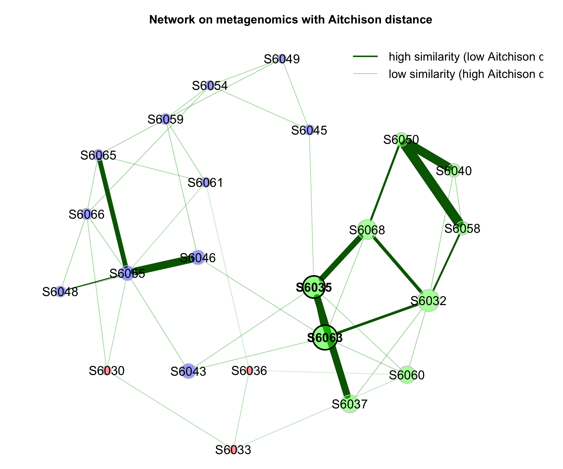
Figure 9.6: Dissimilarity-based Networks
- plot samples with group information
# Get gorup names from the sample table created before
sampletab <- dada2_ps_rare_genus_filter@sam_data %>%
  data.frame()
group_labels <- factor(sampletab$Group)
names(group_labels) <- rownames(sampletab)

# Define group colors
group_lcol <- c("blue3", "red")

plot(props_aitchison,
     layout = "spring",
     repulsion = 0.84,
     shortenLabels = "none",
     labelScale = FALSE,
     rmSingles = TRUE,
     nodeSize = "eigenvector",
     nodeSizeSpread = 4,
     nodeColor = "feature",
     featVecCol = group_labels,
     colorVec =  group_lcol,
     posCol = "darkturquoise",
     negCol = "orange",
     edgeTranspLow = 0,
     edgeTranspHigh = 40,
     cexNodes = 2,
     cexLabels = 2,
     cexHubLabels = 2.5,
     title1 = "Network on genus level with Aitchison distance",
     showTitle = TRUE,
     cexTitle = 2.3)

# Colors used in the legend should be equally transparent as in the plot
group_transp <- NetCoMi:::colToTransp(group_lcol, 60)

legend(-1.2, 1.2, cex = 2, pt.cex = 2.5, title = "Group:",
       legend = levels(group_labels), col = group_transp, bty = "n", pch = 16)

# get green color with 50% transparency
green2 <- colToTransp("#009900", 40)

legend(0.4, 1.1,
       cex = 1.5,
       legend = c("high similarity (low Aitchison distance)",
                  "low similarity (high Aitchison distance)"),
       lty = 1,
       lwd = c(3, 1),
       col = c("darkgreen", green2),
       bty = "n")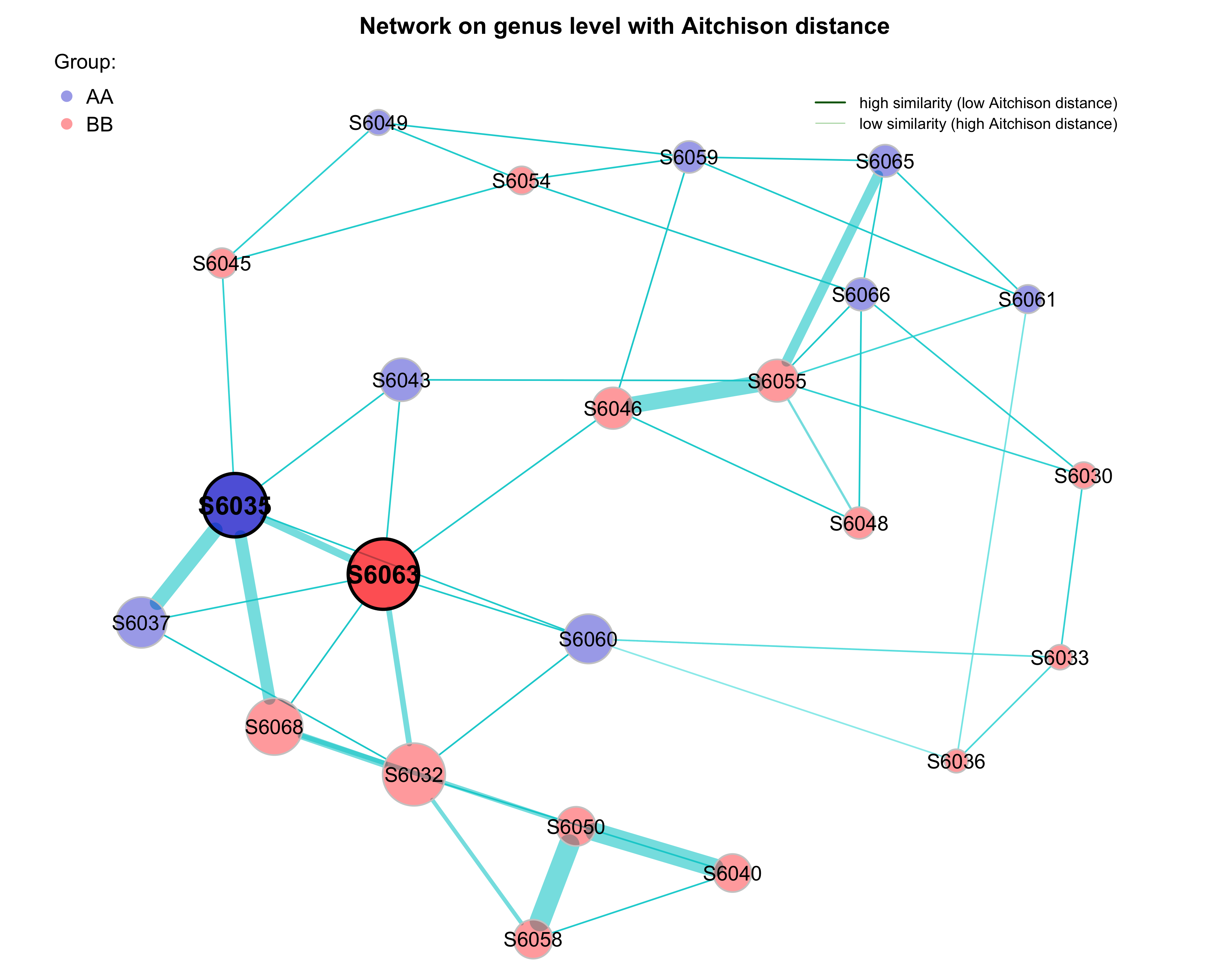
Figure 9.7: Dissimilarity-based Networks (group information)
9.5 Systematic Information
## ─ Session info ───────────────────────────────────────────────────────────────────────────────────────────────────────────────────────────────
## setting value
## version R version 4.1.3 (2022-03-10)
## os macOS Monterey 12.2.1
## system x86_64, darwin17.0
## ui RStudio
## language (EN)
## collate en_US.UTF-8
## ctype en_US.UTF-8
## tz Asia/Shanghai
## date 2023-10-27
## rstudio 2023.09.0+463 Desert Sunflower (desktop)
## pandoc 3.1.1 @ /Applications/RStudio.app/Contents/Resources/app/quarto/bin/tools/ (via rmarkdown)
##
## ─ Packages ───────────────────────────────────────────────────────────────────────────────────────────────────────────────────────────────────
## package * version date (UTC) lib source
## abind 1.4-5 2016-07-21 [2] CRAN (R 4.1.0)
## ade4 1.7-22 2023-02-06 [2] CRAN (R 4.1.2)
## ALDEx2 1.30.0 2022-11-01 [2] Bioconductor
## annotate 1.72.0 2021-10-26 [2] Bioconductor
## AnnotationDbi 1.60.2 2023-03-10 [2] Bioconductor
## ape * 5.7-1 2023-03-13 [2] CRAN (R 4.1.2)
## askpass 1.1 2019-01-13 [2] CRAN (R 4.1.0)
## backports 1.4.1 2021-12-13 [2] CRAN (R 4.1.0)
## base64enc 0.1-3 2015-07-28 [2] CRAN (R 4.1.0)
## bayesm 3.1-5 2022-12-02 [2] CRAN (R 4.1.2)
## Biobase * 2.54.0 2021-10-26 [2] Bioconductor
## BiocGenerics * 0.40.0 2021-10-26 [2] Bioconductor
## BiocParallel 1.28.3 2021-12-09 [2] Bioconductor
## biomformat 1.22.0 2021-10-26 [2] Bioconductor
## Biostrings 2.62.0 2021-10-26 [2] Bioconductor
## bit 4.0.5 2022-11-15 [2] CRAN (R 4.1.2)
## bit64 4.0.5 2020-08-30 [2] CRAN (R 4.1.0)
## bitops 1.0-7 2021-04-24 [2] CRAN (R 4.1.0)
## blob 1.2.4 2023-03-17 [2] CRAN (R 4.1.2)
## bookdown 0.34 2023-05-09 [2] CRAN (R 4.1.2)
## broom 1.0.5 2023-06-09 [2] CRAN (R 4.1.3)
## bslib 0.5.0 2023-06-09 [2] CRAN (R 4.1.3)
## cachem 1.0.8 2023-05-01 [2] CRAN (R 4.1.2)
## callr 3.7.3 2022-11-02 [2] CRAN (R 4.1.2)
## car 3.1-2 2023-03-30 [2] CRAN (R 4.1.2)
## carData 3.0-5 2022-01-06 [2] CRAN (R 4.1.2)
## caTools 1.18.2 2021-03-28 [2] CRAN (R 4.1.0)
## cccd 1.6 2022-04-08 [2] CRAN (R 4.1.2)
## cellranger 1.1.0 2016-07-27 [2] CRAN (R 4.1.0)
## checkmate 2.2.0 2023-04-27 [2] CRAN (R 4.1.2)
## class 7.3-22 2023-05-03 [2] CRAN (R 4.1.2)
## classInt 0.4-9 2023-02-28 [2] CRAN (R 4.1.2)
## cli 3.6.1 2023-03-23 [2] CRAN (R 4.1.2)
## cluster 2.1.4 2022-08-22 [2] CRAN (R 4.1.2)
## coda 0.19-4 2020-09-30 [2] CRAN (R 4.1.0)
## codetools 0.2-19 2023-02-01 [2] CRAN (R 4.1.2)
## coin 1.4-2 2021-10-08 [2] CRAN (R 4.1.0)
## colorspace 2.1-0 2023-01-23 [2] CRAN (R 4.1.2)
## compositions 2.0-6 2023-04-13 [2] CRAN (R 4.1.2)
## conflicted * 1.2.0 2023-02-01 [2] CRAN (R 4.1.2)
## corpcor 1.6.10 2021-09-16 [2] CRAN (R 4.1.0)
## corrplot 0.92 2021-11-18 [2] CRAN (R 4.1.0)
## cowplot 1.1.1 2020-12-30 [2] CRAN (R 4.1.0)
## crayon 1.5.2 2022-09-29 [2] CRAN (R 4.1.2)
## crosstalk 1.2.0 2021-11-04 [2] CRAN (R 4.1.0)
## data.table 1.14.8 2023-02-17 [2] CRAN (R 4.1.2)
## DBI 1.1.3 2022-06-18 [2] CRAN (R 4.1.2)
## DelayedArray 0.20.0 2021-10-26 [2] Bioconductor
## deldir 1.0-9 2023-05-17 [2] CRAN (R 4.1.3)
## DEoptimR 1.0-14 2023-06-09 [2] CRAN (R 4.1.3)
## DESeq2 1.34.0 2021-10-26 [2] Bioconductor
## devtools * 2.4.5 2022-10-11 [2] CRAN (R 4.1.2)
## digest 0.6.33 2023-07-07 [1] CRAN (R 4.1.3)
## doParallel 1.0.17 2022-02-07 [2] CRAN (R 4.1.2)
## doSNOW 1.0.20 2022-02-04 [2] CRAN (R 4.1.2)
## dplyr * 1.1.2 2023-04-20 [2] CRAN (R 4.1.2)
## DT 0.28 2023-05-18 [2] CRAN (R 4.1.3)
## dynamicTreeCut 1.63-1 2016-03-11 [2] CRAN (R 4.1.0)
## e1071 1.7-13 2023-02-01 [2] CRAN (R 4.1.2)
## edgeR 3.36.0 2021-10-26 [2] Bioconductor
## ellipsis 0.3.2 2021-04-29 [2] CRAN (R 4.1.0)
## emmeans 1.8.7 2023-06-23 [1] CRAN (R 4.1.3)
## estimability 1.4.1 2022-08-05 [2] CRAN (R 4.1.2)
## evaluate 0.21 2023-05-05 [2] CRAN (R 4.1.2)
## FactoMineR 2.8 2023-03-27 [2] CRAN (R 4.1.2)
## fansi 1.0.4 2023-01-22 [2] CRAN (R 4.1.2)
## farver 2.1.1 2022-07-06 [2] CRAN (R 4.1.2)
## fastcluster 1.2.3 2021-05-24 [2] CRAN (R 4.1.0)
## fastmap 1.1.1 2023-02-24 [2] CRAN (R 4.1.2)
## fdrtool 1.2.17 2021-11-13 [2] CRAN (R 4.1.0)
## filematrix 1.3 2018-02-27 [2] CRAN (R 4.1.0)
## flashClust 1.01-2 2012-08-21 [2] CRAN (R 4.1.0)
## FNN 1.1.3.2 2023-03-20 [2] CRAN (R 4.1.2)
## foreach 1.5.2 2022-02-02 [2] CRAN (R 4.1.2)
## foreign 0.8-84 2022-12-06 [2] CRAN (R 4.1.2)
## forestplot 3.1.1 2022-12-06 [2] CRAN (R 4.1.2)
## formatR 1.14 2023-01-17 [2] CRAN (R 4.1.2)
## Formula 1.2-5 2023-02-24 [2] CRAN (R 4.1.2)
## fs 1.6.2 2023-04-25 [2] CRAN (R 4.1.2)
## futile.logger * 1.4.3 2016-07-10 [2] CRAN (R 4.1.0)
## futile.options 1.0.1 2018-04-20 [2] CRAN (R 4.1.0)
## genefilter 1.76.0 2021-10-26 [2] Bioconductor
## geneplotter 1.72.0 2021-10-26 [2] Bioconductor
## generics 0.1.3 2022-07-05 [2] CRAN (R 4.1.2)
## GenomeInfoDb * 1.30.1 2022-01-30 [2] Bioconductor
## GenomeInfoDbData 1.2.7 2022-03-09 [2] Bioconductor
## GenomicRanges * 1.46.1 2021-11-18 [2] Bioconductor
## ggiraph 0.8.7 2023-03-17 [2] CRAN (R 4.1.2)
## ggiraphExtra 0.3.0 2020-10-06 [2] CRAN (R 4.1.2)
## ggplot2 * 3.4.2 2023-04-03 [2] CRAN (R 4.1.2)
## ggpubr * 0.6.0 2023-02-10 [2] CRAN (R 4.1.2)
## ggrepel 0.9.3 2023-02-03 [2] CRAN (R 4.1.2)
## ggsci 3.0.0 2023-03-08 [2] CRAN (R 4.1.2)
## ggsignif 0.6.4 2022-10-13 [2] CRAN (R 4.1.2)
## ggVennDiagram 1.2.2 2022-09-08 [2] CRAN (R 4.1.2)
## glasso 1.11 2019-10-01 [2] CRAN (R 4.1.0)
## glmnet 4.1-7 2023-03-23 [2] CRAN (R 4.1.2)
## glue * 1.6.2 2022-02-24 [2] CRAN (R 4.1.2)
## Gmisc * 3.0.2 2023-03-13 [2] CRAN (R 4.1.2)
## GO.db 3.14.0 2022-04-11 [2] Bioconductor
## gplots 3.1.3 2022-04-25 [2] CRAN (R 4.1.2)
## gridExtra 2.3 2017-09-09 [2] CRAN (R 4.1.0)
## gtable 0.3.3 2023-03-21 [2] CRAN (R 4.1.2)
## gtools 3.9.4 2022-11-27 [2] CRAN (R 4.1.2)
## highr 0.10 2022-12-22 [2] CRAN (R 4.1.2)
## Hmisc 5.1-0 2023-05-08 [2] CRAN (R 4.1.2)
## hms 1.1.3 2023-03-21 [2] CRAN (R 4.1.2)
## htmlTable * 2.4.1 2022-07-07 [2] CRAN (R 4.1.2)
## htmltools 0.5.5 2023-03-23 [2] CRAN (R 4.1.2)
## htmlwidgets 1.6.2 2023-03-17 [2] CRAN (R 4.1.2)
## httpuv 1.6.11 2023-05-11 [2] CRAN (R 4.1.3)
## httr 1.4.6 2023-05-08 [2] CRAN (R 4.1.2)
## huge 1.3.5 2021-06-30 [2] CRAN (R 4.1.0)
## igraph 1.5.0 2023-06-16 [1] CRAN (R 4.1.3)
## impute 1.68.0 2021-10-26 [2] Bioconductor
## insight 0.19.3 2023-06-29 [2] CRAN (R 4.1.3)
## IRanges * 2.28.0 2021-10-26 [2] Bioconductor
## irlba 2.3.5.1 2022-10-03 [2] CRAN (R 4.1.2)
## iterators 1.0.14 2022-02-05 [2] CRAN (R 4.1.2)
## jpeg 0.1-10 2022-11-29 [2] CRAN (R 4.1.2)
## jquerylib 0.1.4 2021-04-26 [2] CRAN (R 4.1.0)
## jsonlite 1.8.7 2023-06-29 [2] CRAN (R 4.1.3)
## kableExtra 1.3.4 2021-02-20 [2] CRAN (R 4.1.2)
## KEGGREST 1.34.0 2021-10-26 [2] Bioconductor
## KernSmooth 2.23-22 2023-07-10 [2] CRAN (R 4.1.3)
## knitr 1.43 2023-05-25 [2] CRAN (R 4.1.3)
## labeling 0.4.2 2020-10-20 [2] CRAN (R 4.1.0)
## lambda.r 1.2.4 2019-09-18 [2] CRAN (R 4.1.0)
## later 1.3.1 2023-05-02 [2] CRAN (R 4.1.2)
## lattice * 0.21-8 2023-04-05 [2] CRAN (R 4.1.2)
## lavaan 0.6-15 2023-03-14 [2] CRAN (R 4.1.2)
## leaps 3.1 2020-01-16 [2] CRAN (R 4.1.0)
## libcoin 1.0-9 2021-09-27 [2] CRAN (R 4.1.0)
## lifecycle 1.0.3 2022-10-07 [2] CRAN (R 4.1.2)
## limma 3.50.3 2022-04-07 [2] Bioconductor
## locfit 1.5-9.8 2023-06-11 [2] CRAN (R 4.1.3)
## LOCOM 1.1 2022-08-05 [2] Github (yijuanhu/LOCOM@c181e0f)
## lubridate 1.9.2 2023-02-10 [2] CRAN (R 4.1.2)
## magrittr * 2.0.3 2022-03-30 [2] CRAN (R 4.1.2)
## MASS 7.3-60 2023-05-04 [2] CRAN (R 4.1.2)
## Matrix 1.6-0 2023-07-08 [2] CRAN (R 4.1.3)
## MatrixGenerics * 1.6.0 2021-10-26 [2] Bioconductor
## matrixStats * 1.0.0 2023-06-02 [2] CRAN (R 4.1.3)
## mbzinb 0.2 2022-03-16 [2] local
## memoise 2.0.1 2021-11-26 [2] CRAN (R 4.1.0)
## metagenomeSeq 1.36.0 2021-10-26 [2] Bioconductor
## mgcv 1.8-42 2023-03-02 [2] CRAN (R 4.1.2)
## microbiome 1.16.0 2021-10-26 [2] Bioconductor
## mime 0.12 2021-09-28 [2] CRAN (R 4.1.0)
## miniUI 0.1.1.1 2018-05-18 [2] CRAN (R 4.1.0)
## mixedCCA 1.6.2 2022-09-09 [2] CRAN (R 4.1.2)
## mnormt 2.1.1 2022-09-26 [2] CRAN (R 4.1.2)
## modeltools 0.2-23 2020-03-05 [2] CRAN (R 4.1.0)
## multcomp 1.4-25 2023-06-20 [2] CRAN (R 4.1.3)
## multcompView 0.1-9 2023-04-09 [2] CRAN (R 4.1.2)
## multtest 2.50.0 2021-10-26 [2] Bioconductor
## munsell 0.5.0 2018-06-12 [2] CRAN (R 4.1.0)
## mvtnorm 1.2-2 2023-06-08 [2] CRAN (R 4.1.3)
## mycor 0.1.1 2018-04-10 [2] CRAN (R 4.1.0)
## NADA 1.6-1.1 2020-03-22 [2] CRAN (R 4.1.0)
## NetCoMi * 1.0.3 2022-07-14 [2] Github (stefpeschel/NetCoMi@d4d80d3)
## nlme * 3.1-162 2023-01-31 [2] CRAN (R 4.1.2)
## nnet 7.3-19 2023-05-03 [2] CRAN (R 4.1.2)
## openssl 2.0.6 2023-03-09 [2] CRAN (R 4.1.2)
## pbapply 1.7-2 2023-06-27 [2] CRAN (R 4.1.3)
## pbivnorm 0.6.0 2015-01-23 [2] CRAN (R 4.1.0)
## pcaPP 2.0-3 2022-10-24 [2] CRAN (R 4.1.2)
## permute * 0.9-7 2022-01-27 [2] CRAN (R 4.1.2)
## pheatmap * 1.0.12 2019-01-04 [2] CRAN (R 4.1.0)
## phyloseq * 1.38.0 2021-10-26 [2] Bioconductor
## picante * 1.8.2 2020-06-10 [2] CRAN (R 4.1.0)
## pillar 1.9.0 2023-03-22 [2] CRAN (R 4.1.2)
## pkgbuild 1.4.2 2023-06-26 [2] CRAN (R 4.1.3)
## pkgconfig 2.0.3 2019-09-22 [2] CRAN (R 4.1.0)
## pkgload 1.3.2.1 2023-07-08 [2] CRAN (R 4.1.3)
## plyr 1.8.8 2022-11-11 [2] CRAN (R 4.1.2)
## png 0.1-8 2022-11-29 [2] CRAN (R 4.1.2)
## ppcor 1.1 2015-12-03 [2] CRAN (R 4.1.0)
## preprocessCore 1.56.0 2021-10-26 [2] Bioconductor
## prettyunits 1.1.1 2020-01-24 [2] CRAN (R 4.1.0)
## processx 3.8.2 2023-06-30 [2] CRAN (R 4.1.3)
## profvis 0.3.8 2023-05-02 [2] CRAN (R 4.1.2)
## promises 1.2.0.1 2021-02-11 [2] CRAN (R 4.1.0)
## protoclust 1.6.4 2022-04-01 [2] CRAN (R 4.1.2)
## proxy 0.4-27 2022-06-09 [2] CRAN (R 4.1.2)
## ps 1.7.5 2023-04-18 [2] CRAN (R 4.1.2)
## pscl 1.5.5.1 2023-05-10 [2] CRAN (R 4.1.2)
## psych 2.3.6 2023-06-21 [2] CRAN (R 4.1.3)
## pulsar 0.3.10 2023-01-26 [2] CRAN (R 4.1.2)
## purrr * 1.0.1 2023-01-10 [2] CRAN (R 4.1.2)
## qgraph 1.9.5 2023-05-16 [2] CRAN (R 4.1.3)
## quadprog 1.5-8 2019-11-20 [2] CRAN (R 4.1.0)
## qvalue 2.26.0 2021-10-26 [2] Bioconductor
## R6 2.5.1 2021-08-19 [2] CRAN (R 4.1.0)
## RAIDA 1.0 2022-03-14 [2] local
## rbibutils 2.2.13 2023-01-13 [2] CRAN (R 4.1.2)
## RColorBrewer * 1.1-3 2022-04-03 [2] CRAN (R 4.1.2)
## Rcpp * 1.0.11 2023-07-06 [1] CRAN (R 4.1.3)
## RcppZiggurat 0.1.6 2020-10-20 [2] CRAN (R 4.1.0)
## RCurl 1.98-1.12 2023-03-27 [2] CRAN (R 4.1.2)
## Rdpack 2.4 2022-07-20 [2] CRAN (R 4.1.2)
## readr * 2.1.4 2023-02-10 [2] CRAN (R 4.1.2)
## readxl * 1.4.3 2023-07-06 [2] CRAN (R 4.1.3)
## remotes 2.4.2 2021-11-30 [2] CRAN (R 4.1.0)
## reshape2 1.4.4 2020-04-09 [2] CRAN (R 4.1.0)
## reticulate 1.30 2023-06-09 [2] CRAN (R 4.1.3)
## Rfast 2.0.8 2023-07-03 [2] CRAN (R 4.1.3)
## rhdf5 2.38.1 2022-03-10 [2] Bioconductor
## rhdf5filters 1.6.0 2021-10-26 [2] Bioconductor
## Rhdf5lib 1.16.0 2021-10-26 [2] Bioconductor
## rlang 1.1.1 2023-04-28 [1] CRAN (R 4.1.2)
## rmarkdown 2.23 2023-07-01 [2] CRAN (R 4.1.3)
## robustbase 0.99-0 2023-06-16 [2] CRAN (R 4.1.3)
## rootSolve 1.8.2.3 2021-09-29 [2] CRAN (R 4.1.0)
## rpart 4.1.19 2022-10-21 [2] CRAN (R 4.1.2)
## RSpectra 0.16-1 2022-04-24 [2] CRAN (R 4.1.2)
## RSQLite 2.3.1 2023-04-03 [2] CRAN (R 4.1.2)
## rstatix 0.7.2 2023-02-01 [2] CRAN (R 4.1.2)
## rstudioapi 0.15.0 2023-07-07 [2] CRAN (R 4.1.3)
## Rtsne 0.16 2022-04-17 [2] CRAN (R 4.1.2)
## RVenn 1.1.0 2019-07-18 [2] CRAN (R 4.1.0)
## rvest 1.0.3 2022-08-19 [2] CRAN (R 4.1.2)
## S4Vectors * 0.32.4 2022-03-29 [2] Bioconductor
## sandwich 3.0-2 2022-06-15 [2] CRAN (R 4.1.2)
## sass 0.4.6 2023-05-03 [2] CRAN (R 4.1.2)
## scales 1.2.1 2022-08-20 [2] CRAN (R 4.1.2)
## scatterplot3d 0.3-44 2023-05-05 [2] CRAN (R 4.1.2)
## sessioninfo 1.2.2 2021-12-06 [2] CRAN (R 4.1.0)
## sf 1.0-7 2022-03-07 [2] CRAN (R 4.1.2)
## shape 1.4.6 2021-05-19 [2] CRAN (R 4.1.0)
## shiny 1.7.4.1 2023-07-06 [2] CRAN (R 4.1.3)
## sjlabelled 1.2.0 2022-04-10 [2] CRAN (R 4.1.2)
## sjmisc 2.8.9 2021-12-03 [2] CRAN (R 4.1.0)
## snow 0.4-4 2021-10-27 [2] CRAN (R 4.1.0)
## SpiecEasi * 1.1.2 2022-07-14 [2] Github (zdk123/SpiecEasi@c463727)
## SPRING 1.0.4 2022-08-03 [2] Github (GraceYoon/SPRING@3d641a4)
## stringi 1.7.12 2023-01-11 [2] CRAN (R 4.1.2)
## stringr 1.5.0 2022-12-02 [2] CRAN (R 4.1.2)
## SummarizedExperiment * 1.24.0 2021-10-26 [2] Bioconductor
## survival 3.5-5 2023-03-12 [2] CRAN (R 4.1.2)
## svglite 2.1.1 2023-01-10 [2] CRAN (R 4.1.2)
## systemfonts 1.0.4 2022-02-11 [2] CRAN (R 4.1.2)
## tensorA 0.36.2 2020-11-19 [2] CRAN (R 4.1.0)
## TH.data 1.1-2 2023-04-17 [2] CRAN (R 4.1.2)
## tibble * 3.2.1 2023-03-20 [2] CRAN (R 4.1.2)
## tidyr * 1.3.0 2023-01-24 [2] CRAN (R 4.1.2)
## tidyselect 1.2.0 2022-10-10 [2] CRAN (R 4.1.2)
## timechange 0.2.0 2023-01-11 [2] CRAN (R 4.1.2)
## truncnorm 1.0-9 2023-03-20 [2] CRAN (R 4.1.2)
## tzdb 0.4.0 2023-05-12 [2] CRAN (R 4.1.3)
## umap 0.2.10.0 2023-02-01 [2] CRAN (R 4.1.2)
## units 0.8-2 2023-04-27 [2] CRAN (R 4.1.2)
## urlchecker 1.0.1 2021-11-30 [2] CRAN (R 4.1.0)
## usethis * 2.2.2 2023-07-06 [2] CRAN (R 4.1.3)
## utf8 1.2.3 2023-01-31 [2] CRAN (R 4.1.2)
## uuid 1.1-0 2022-04-19 [2] CRAN (R 4.1.2)
## vctrs 0.6.3 2023-06-14 [1] CRAN (R 4.1.3)
## vegan * 2.6-4 2022-10-11 [2] CRAN (R 4.1.2)
## VennDiagram * 1.7.3 2022-04-12 [2] CRAN (R 4.1.2)
## VGAM 1.1-8 2023-03-09 [2] CRAN (R 4.1.2)
## viridis * 0.6.3 2023-05-03 [2] CRAN (R 4.1.2)
## viridisLite * 0.4.2 2023-05-02 [2] CRAN (R 4.1.2)
## vroom 1.6.3 2023-04-28 [2] CRAN (R 4.1.2)
## webshot 0.5.5 2023-06-26 [2] CRAN (R 4.1.3)
## WGCNA 1.72-1 2023-01-18 [2] CRAN (R 4.1.2)
## withr 2.5.0 2022-03-03 [2] CRAN (R 4.1.2)
## Wrench 1.12.0 2021-10-26 [2] Bioconductor
## xfun 0.40 2023-08-09 [1] CRAN (R 4.1.3)
## XMAS2 * 2.2.0 2023-10-27 [1] local
## XML 3.99-0.14 2023-03-19 [2] CRAN (R 4.1.2)
## xml2 1.3.5 2023-07-06 [2] CRAN (R 4.1.3)
## xtable 1.8-4 2019-04-21 [2] CRAN (R 4.1.0)
## XVector 0.34.0 2021-10-26 [2] Bioconductor
## yaml 2.3.7 2023-01-23 [2] CRAN (R 4.1.2)
## zCompositions 1.4.0-1 2022-03-26 [2] CRAN (R 4.1.2)
## zlibbioc 1.40.0 2021-10-26 [2] Bioconductor
## zoo 1.8-12 2023-04-13 [2] CRAN (R 4.1.2)
##
## [1] /Users/zouhua/Library/R/x86_64/4.1/library
## [2] /Library/Frameworks/R.framework/Versions/4.1/Resources/library
##
## ──────────────────────────────────────────────────────────────────────────────────────────────────────────────────────────────────────────────